A one-sample z-test is used to compare a sample proportion to a population proportion. The document provides an example where a survey claims 90% of doctors recommend aspirin, and a sample of 100 doctors found 82% recommend aspirin. The z-test is calculated to determine if this difference is statistically significant. The null hypothesis is the sample and population proportions are the same. If the calculated z-statistic falls outside the critical values of -1.96 and 1.96, the null will be rejected, meaning the proportions are significantly different.

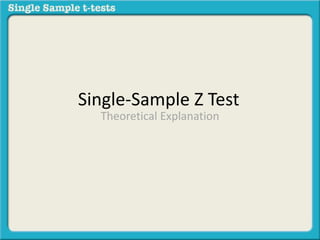
1. Single-Sample Z Test
Theoretical Explanation

2. A one-sample Z-test for proportions is a test that helps
us compare a population proportion with a sample
proportion.

3. A one-sample Z-test for proportions is a test that helps
us compare a population proportion with a sample
proportion.
30%
Sample Mean
(푋 )
30%
Population Mean
(휇)

4. A one-sample Z-test for proportions is a test that helps
us compare a population proportion with a sample
proportion.
This is the
symbol for
a sample
mean
30%
Sample Mean
( 푿)
30%
Population Mean
(휇)

5. A one-sample Z-test for proportions is a test that helps
us compare a population proportion with a sample
proportion.
And this is the
symbol for a
population mean
(called a mew)
30%
Sample Mean
(푋 )
30%
Population Mean
(흁)

6. A one-sample Z-test for proportions is a test that helps
us compare a population proportion with a sample
proportion.
30%
Sample Mean
(푋 )
Here is our question:
30%
Population Mean
(휇)

7. A one-sample Z-test for proportions is a test that helps
us compare a population proportion with a sample
proportion.
30%
Sample Mean
(푋 )
30%
Population Mean
(휇)
Here is our question: Are the population and the
sample proportions (which supposedly have the same
general characteristics as the population) statistically
significantly the same or different?

8. Consider the following example:

9. Consider the following example:
A survey claims that 9 out of 10 doctors recommend
aspirin for their patients with headaches. To test this
claim, a random sample of 100 doctors is obtained. Of
these 100 doctors, 82 indicate that they recommend
aspirin. Is this claim accurate? Use alpha = 0.05

10. Consider the following example:
A survey claims that 9 out of 10 doctors recommend
aspirin for their patients with headaches. To test this
claim, a random sample of 100 doctors is obtained. Of
these 100 doctors, 82 indicate that they recommend
aspirin. Is this claim accurate? Use alpha = 0.05
Which is the sample?

11. Consider the following example:
A survey claims that 9 out of 10 doctors recommend
aspirin for their patients with headaches. To test this
claim, a random sample of 100 doctors is obtained. Of
these 100 doctors, 82 indicate that they recommend
aspirin. Is this claim accurate? Use alpha = 0.05
Which is the sample?
What is the population?

12. Consider the following example:
A survey claims that 9 out of 10 doctors recommend
aspirin for their patients with headaches. To test this
claim, a random sample of 100 doctors is obtained. Of
these 100 doctors, 82 indicate that they recommend
aspirin. Is this claim accurate? Use alpha = 0.05
Which is the sample?
What is the population?
The sample proportion is .82 doctors recommending
aspirin.

13. Consider the following example:
A survey claims that 9 out of 10 doctors recommend
aspirin for their patients with headaches. To test this
claim, a random sample of 100 doctors is obtained. Of
these 100 doctors, 82 indicate that they recommend
aspirin. Is this claim accurate? Use alpha = 0.05
Which is the sample?
What is the population?
The sample proportion is .82 of doctors recommending
aspirin.
The population proportion .90 (the claim that 9 out of
10 doctors recommend aspirin).

14. We begin by stating the null hypothesis:

15. We begin by stating the null hypothesis:
The proportion of a sample of 100 medical doctors who
recommend aspirin for their patients with headaches IS NOT
statistically significantly different from the claim that 9 out of
10 doctors recommend aspirin for their patients with
headaches.

16. We begin by stating the null hypothesis:
The proportion of a sample of 100 medical doctors who
recommend aspirin for their patients with headaches IS NOT
statistically significantly different from the claim that 9 out of
10 doctors recommend aspirin for their patients with
headaches.
The alternative hypothesis would be:

17. We begin by stating the null hypothesis:
The proportion of a sample of 100 medical doctors who
recommend aspirin for their patients with headaches IS NOT
statistically significantly different from the claim that 9 out of
10 doctors recommend aspirin for their patients with
headaches.
The alternative hypothesis would be:
The proportion of a sample of 100 medical doctors who
recommend aspirin for their patients with headaches IS
statistically significantly different from the claim that 9 out of
10 doctors recommend aspirin for their patients with
headaches.

18. State the decision rule:

19. State the decision rule: We will calculate what is called
the z statistic which will make it possible to determine
the likelihood that the sample proportion (.82) is a rare
or common occurrence with reference to the
population proportion (.90).

20. State the decision rule: We will calculate what is called
the z statistic which will make it possible to determine
the likelihood that the sample proportion (.82) is a rare
or common occurrence with reference to the
population proportion (.90).
If the z-statistic falls outside of the 95% common
occurrences and into the 5% rare occurrences then we
will conclude that it is a rare event and that the sample
is different from the population and therefore reject
the null hypothesis.

21. Before we calculate this z-statistic, we must locate the
z critical values.

22. Before we calculate this z-statistic, we must locate the
z critical values.
What are the z critical values? These are the values
that demarcate what is the rare and the common
occurrence.

23. Let’s look at the normal distribution:
It has some important properties that make it possible
for us to locate the z statistic and compare it to the z
critical.

24. Here is the mean and the median of a normal
distribution.

25. 50% of the values are above and below the orange
line.
50% - 50% +

26. 68% of the values fall between +1 and -1 standard
deviations from the mean.
34% - 34% +

27. 68% of the values fall between +1 and -1 standard
deviations from the mean.
34% - 34% +
-1σ mean +1σ
68%

28. 68% of the values fall between +1 and -1 standard
deviations from the mean.
34% - 34% +
-2σ -1σ mean +1σ +2σ
95%

29. Since our decision rule is .05 alpha, this means that if
the z value falls outside of the 95% common
occurrences we will consider it a rare occurrence.
34% - 34% +
-2σ -1σ mean +1σ +2σ
95%

30. Since are decision rule is .05 alpha we will see if the z
statistic is rare using this visual
rare rare
-2σ -1σ mean +1σ +2σ
2.5% 95%
2.5%

31. Or common
Common
-2σ -1σ mean +1σ +2σ
95%

32. Before we can calculate the z – statistic to see if it is
rare or common we first must determine the z critical
values that are associated with -2σ and +2σ.
Common
-2σ -1σ mean +1σ +2σ
95%

33. We look these up in the Z table and find that they are -
1.96 and +1.96
Common
-2σ -1σ mean +1σ +2σ
Z values -1.96 +1.96
95%

34. So if the z statistic we calculate is less than -1.96
(e.g., -1.99) or greater than +1.96 (e.g., +2.30) then we
will consider this to be a rare event and reject the null
hypothesis and state that there is a statistically
significant difference between .9 (population) and .82
(the sample).

35. So if the z statistic we calculate is less than -1.96
(e.g., -1.99) or greater than +1.96 (e.g., +2.30) then we
will consider this to be a rare event and reject the null
hypothesis and state that there is a statistically
significant difference between .9 (population) and .82
(the sample).
Let’s calculate the z statistic and see where if falls!

36. So if the z statistic we calculate is less than -1.96
(e.g., -1.99) or greater than +1.96 (e.g., +2.30) then we
will consider this to be a rare event and reject the null
hypothesis and state that there is a statistically
significant difference between .9 (population) and .82
(the sample).
Let’s calculate the z statistic and see where if falls!
We do this by using the following equation:

37. So if the z statistic we calculate is less than -1.96
(e.g., -1.99) or greater than +1.96 (e.g., +2.30) then we
will consider this to be a rare event and reject the null
hypothesis and state that there is a statistically
significant difference between .9 (population) and .82
(the sample).
Let’s calculate the z statistic and see where if falls!
We do this by using the following equation:
풛풔풕풂풕풊풔풕풊풄 =
푝 − 푝
푝(1 − 푝)
푛

38. So if the z statistic we calculate is less than -1.96
(e.g., -1.99) or greater than +1.96 (e.g., +2.30) then we
will consider this to be a rare event and reject the null
hypothesis and state that there is a statistically
significant difference between .9 (population) and .82
(the sample).
Let’s calculate the z statistic and see where if falls!
We do this by using the following equation:
풛풔풕풂풕풊풔풕풊풄 =
푝 − 푝
푝(1 − 푝)
푛
Zstatistic is what we are trying to find to see if it is
outside or inside the z critical values (-1.96 and +1.96).

39. Here’s the problem again:

40. A survey claims that 9 out of 10 doctors recommend aspirin for
their patients with headaches. To test this claim, a random
sample of 100 doctors is obtained. Of these 100 doctors, 82
indicate that they recommend aspirin. Is this claim accurate?
Use alpha = 0.05

41. A survey claims that 9 out of 10 doctors recommend aspirin for
their patients with headaches. To test this claim, a random
sample of 100 doctors is obtained. Of these 100 doctors, 82
indicate that they recommend aspirin. Is this claim accurate?
Use alpha = 0.05

42. 풑 is the proportion from the sample that
recommended aspirin to their patients (. ퟖퟐ)
풛풔풕풂풕풊풔풕풊풄 =
푝 − 푝
푝(1 − 푝)
푛

43. 풑 is the proportion from the sample that
recommended aspirin to their patients (. ퟖퟐ)
풛풔풕풂풕풊풔풕풊풄 =
푝 − 푝
푝(1 − 푝)
푛
Note – this little
hat (푝 ) over the
p means that
this proportion
is an estimate
of a population

44. 퐩 is the proportion from the population that
recommended aspirin to their patients (.90)
풛풔풕풂풕풊풔풕풊풄 =
푝 − 푝
푝(1 − 푝)
푛

45. 풏 is the size of the sample (100)
풛풔풕풂풕풊풔풕풊풄 =
푝 − 푝
푝(1 − 푝)
푛

46. A survey claims that 9 out of 10 doctors recommend aspirin for
their patients with headaches. To test this claim, a random
sample of 100 doctors is obtained. Of these 100 doctors, 82
indicate that they recommend aspirin. Is this claim accurate?
Use alpha = 0.05
풏 is the size of the sample (100)
풛풔풕풂풕풊풔풕풊풄 =
푝 − 푝
푝(1 − 푝)
푛

47. A survey claims that 9 out of 10 doctors recommend aspirin for
their patients with headaches. To test this claim, a random
sample of 100 doctors is obtained. Of these 100 doctors, 82
indicate that they recommend aspirin. Is this claim accurate?
Use alpha = 0.05
풏 is the size of the sample (100)
풛풔풕풂풕풊풔풕풊풄 =
푝 − 푝
푝(1 − 푝)
푛

48. 풛풔풕풂풕풊풔풕풊풄 =
푝 − 푝
푝(1 − 푝)
푛
Let’s plug in the numbers

49. 풛풔풕풂풕풊풔풕풊풄 =
.82 − 푝
푝(1 − 푝)
푛
Sample Proportion

50. A survey claims that 9 out of 10 doctors recommend aspirin for
their patients with headaches. To test this claim, a random
sample of 100 doctors is obtained. Of these 100 doctors, 82
indicate that they recommend aspirin. Is this claim accurate?
Use alpha = 0.05
풛풔풕풂풕풊풔풕풊풄 =
.82 − 푝
푝(1 − 푝)
푛
Sample Proportion

51. A survey claims that 9 out of 10 doctors recommend aspirin for
their patients with headaches. To test this claim, a random
sample of 100 doctors is obtained. Of these 100 doctors, 82
indicate that they recommend aspirin. Is this claim accurate?
Use alpha = 0.05
풛풔풕풂풕풊풔풕풊풄 =
.82 − 푝
푝(1 − 푝)
푛
Sample Proportion

52. 풛풔풕풂풕풊풔풕풊풄 =
.82 − .90
.90(1 − .90)
푛
Population Proportion

53. A survey claims that 9 out of 10 doctors recommend aspirin for
their patients with headaches. To test this claim, a random
sample of 100 doctors is obtained. Of these 100 doctors, 82
indicate that they recommend aspirin. Is this claim accurate?
Use alpha = 0.05
풛풔풕풂풕풊풔풕풊풄 =
.82 − .90
.90(1 − .90)
푛
Population Proportion

54. A survey claims that 9 out of 10 doctors recommend aspirin for
their patients with headaches. To test this claim, a random
sample of 100 doctors is obtained. Of these 100 doctors, 82
indicate that they recommend aspirin. Is this claim accurate?
Use alpha = 0.05
풛풔풕풂풕풊풔풕풊풄 =
.82 − .90
.90(1 − .90)
푛
Population Proportion

55. The difference
풛풔풕풂풕풊풔풕풊풄 =
.82 − .90
.90(1 − .90)
푛

56. 풛풔풕풂풕풊풔풕풊풄 =
−.08
.90(1 − .90)
푛
The difference

57. Now for the denominator which is the estimated
standard error. This value will help us know how many
standard error units .82 and .90 are apart from one
another (we already know they are .08 raw units apart)

58. Now for the denominator which is the estimated
standard error. This value will help us know how many
standard error units .82 and .90 are apart from one
another (we already know they are .08 raw units apart)
풛풔풕풂풕풊풔풕풊풄 =
−.08
.90(1 − .90)
푛

59. Note - If the standard error is small then the z statistic
will be larger. The larger the z statistics the more likely
that it will exceed the -1.96 or +1.96 boundaries,
compelling us to reject the null hypothesis. If it is
smaller than we will not.
풛풔풕풂풕풊풔풕풊풄 =
−.08
.90(1 − .90)
푛

60. Let’s continue our calculations and find out:
풛풔풕풂풕풊풔풕풊풄 =
−.08
.90(1 − .90)
푛

61. A survey claims that 9 out of 10 doctors recommend aspirin for
their patients with headaches. To test this claim, a random
sample of 100 doctors is obtained. Of these 100 doctors, 82
indicate that they recommend aspirin. Is this claim accurate?
Use alpha = 0.05
Let’s continue our calculations and find out:
풛풔풕풂풕풊풔풕풊풄 =
−.08
.90(1 − .90)
푛

62. Let’s continue our calculations and find out:
풛풔풕풂풕풊풔풕풊풄 =
−.08
.90(.10)
푛

63. Let’s continue our calculations and find out:
풛풔풕풂풕풊풔풕풊풄 =
−.08
.09
푛

64. 풛풔풕풂풕풊풔풕풊풄 =
−.08
.09
100
Sample Size:

65. A survey claims that 9 out of 10 doctors recommend aspirin for
their patients with headaches. To test this claim, a random
sample of 100 doctors is obtained. Of these 100 doctors, 82
indicate that they recommend aspirin. Is this claim accurate?
Use alpha = 0.05
풛풔풕풂풕풊풔풕풊풄 =
−.08
.09
100
Sample Size:

66. Let‘s continue our calculations:
풛풔풕풂풕풊풔풕풊풄 =
−.08
.0009

67. Let‘s continue our calculations:
풛풔풕풂풕풊풔풕풊풄 =
−.08
.03

68. Let‘s continue our calculations:
풛풔풕풂풕풊풔풕풊풄 = −2.67

69. Let‘s continue our calculations:
풛풔풕풂풕풊풔풕풊풄 = −2.67
Now we have our z statistic.

70. Let’s go back to our distribution:
Common
rare rare
-2σ -1σ mean +1σ +2σ
-1.96 +1.96
95%

71. Let’s go back to our distribution: So, is this result
rare or common?
Common
rare rare
-2σ -1σ mean +1σ +2σ
-2.67 -1.96 +1.96
95%

72. Let’s go back to our distribution: So, is this result
rare or common?
Common
rare rare
-2σ -1σ mean +1σ +2σ
-1.96 +1.96
95%
-2.67
This is the
Z-Statistic we
calculated

73. Let’s go back to our distribution: So, is this result
rare or common?
Common
rare rare
-2σ -1σ mean +1σ +2σ
-2.67 -1.96 +1.96
95%
This is the
Z – Critical

74. Looks like it is a rare event therefore we will reject the
null hypothesis in favor of the alternative hypothesis:

75. Looks like it is a rare event therefore we will reject the
null hypothesis in favor of the alternative hypothesis:
The proportion of a sample of 100 medical doctors
who recommend aspirin for their patients with
headaches IS statistically significantly different from
the claim that 9 out of 10 doctors recommend aspirin
for their patients with headaches.