Downloaded 102 times


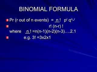
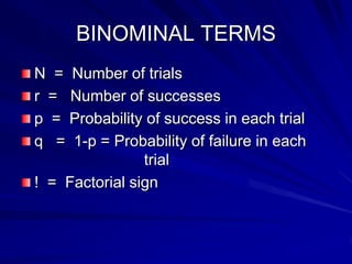


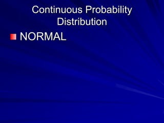
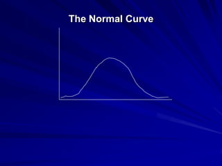


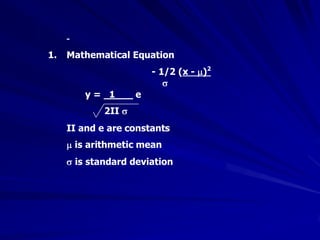
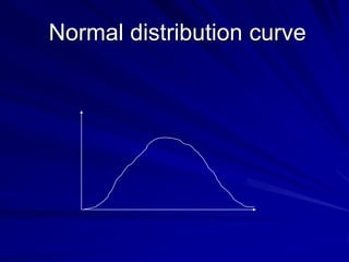
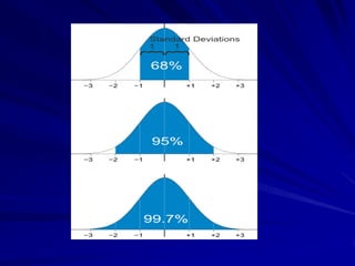

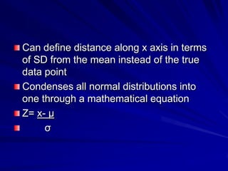


This document provides an overview of probability theory, including key definitions, concepts, and calculations. It discusses: 1. Definitions of probability, including the frequency and subjective concepts. It also defines basic terminology like experiments, trials, outcomes, and events. 2. Methods of calculating probability, including classical and empirical approaches. It presents the classical probability formula. 3. Common probability distributions like the binomial distribution and normal distribution. It provides examples of calculating probabilities using these distributions. 4. Additional probability concepts like independent and conditional probability, random variables, and transformations to the standardized normal distribution. 5. The importance of the normal distribution in applications like medicine, sampling, and statistical significance testing. It


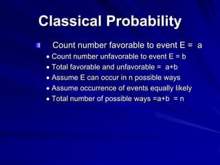
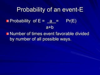
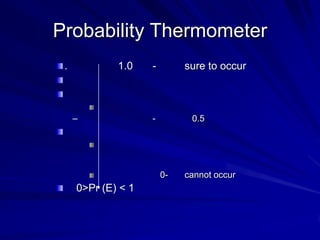
![ch_5-8_probability155[1].ppt](https://cdn.slidesharecdn.com/ss_thumbnails/ch5-8probability1551-231116061842-b428d0bc-thumbnail.jpg?width=640&height=640&fit=bounds)


