Chapter 3

STT 200
STATISTICAL METHODS
Chapter 3: Foundation for
Inference

3.1 Inference for a Single Proportion
■ Trial: A single experiment that leads to an outcome
■ Binomial trial: A trial that has just two possible outcomes
1. Success: the outcome you are keeping track of or
counting out or interested in
■ Denoted by 1
2. Failure: the other outcome
■ Denoted by 0
■ The sample proportion is the mean of the 1s and 0s.
– For example: Proportion of rotten eggs out of 10
eggs. Here success is finding a rotten egg!
Ƹ𝑝 =
1 + 1 + 0 + 1 + 0 + 0 + 0 + 1 + 1 + 1
10
= 0.6
2

Using the normal model for a sample proportion
■ The distribution of all possible sample statistics/proportions Ƹ𝑝
for a given population parameter/proportion value p is called
the sampling distribution.
■ Central Limit Theorem: The sampling distribution for Ƹ𝑝 can be
approximated by a normal distribution in two cases and if two
conditions are satisfied.
■ Case 1: A random sample is taken from a relatively large
population, and a binomial trait is recorded.
■ Case 2: A binomial experiment is repeated numerous times.
■ Condition #1: observations are independent (equivalently the
data is from a random sample)
■ Condition #2: the “expected success/failure” condition
3

Expected success/failure condition: What is this?
■ Recall that p is the probability of success or the population proportion.
Example:
■ Roll a fair die 120 times, then how many “sixes” do you expect to show
up? TOP HAT
■ How many “NOT sixes” do you expect to show up?
■ 𝒏p is the expected number of successes, and this must be at least 10
■ 𝒏(𝟏 − 𝒑) is the expected number of failures, and this must also be at
least 10
■ This makes the sampling distribution symmetrical and the normal curve
a good approximation for the sampling distribution.
■ Condition #2 (in box on PAGE 97)
Our sample must be large enough that we must expect to see at least 10
successes and 10 failures in our sample. That is,
𝑛𝑝 ≥ 10 𝑎𝑛𝑑 𝑛(1 − 𝑝) ≥ 10
4

Normal distribution as sampling distribution
We are at Bottom PAGE 97
■ If these conditions are met, then the sampling distribution of
sample proportions Ƹ𝑝 is nearly normal.
■ The mean of this normal distribution is p, the population
proportion.
■ The standard deviation of the sampling distribution of Ƹ𝑝 is
called the standard error and is calculated using the formula:
𝑆𝐸ො𝑝 =
𝑝 1−𝑝
𝑛
, where 𝑝 is the population proportion which is
usually unknown and will have to be estimated.
■ We can interpret the standard error as approximately the
average distance of the possible Ƹ𝑝 values from the population
proportion, 𝑝, for repeated samples of size 𝑛.
5

Example: B+ Blood (1)
■ 10% of adults have a B+ blood-type.
■ Suppose a random sample of 180 adults is selected and their blood type
recorded. Let ො𝑝 represent the proportion of this 180-person sample who have
B+ blood.
■ Provide a sketch of the normal model we could
use to approximate the distribution of the
sample proportion ො𝑝.
■ Mean = 0.10, note population proportion
is the mean
■ SE=
𝟎.𝟏×(𝟏−𝟎.𝟏)
𝟏𝟖𝟎
= 𝟎. 𝟎𝟐𝟐𝟑𝟔,
here we use p=0.1 to find it.
1. How likely would it be for the sample
proportion ො𝑝 to fall further than
4% (0.04) from the population
proportion 𝑝 = 0.10?
Answer: Further than 4% from 0.10 means less than 0.06 or more than 0.14. So, the
probability we want is
2 x normalcdf(0.14, 𝟏𝟎 𝟏𝟎
, 0.1, 0.02236) = 0.07363
6

■ Suppose a random sample of 180 adults is selected and
their blood type recorded.
■ Let Ƹ𝑝 represent the proportion of this 180-person
sample who have B+ blood.
2. Complete the following sentence:
If we took repeated random samples of 180 individuals, we
would expect Ƹ𝑝 to fall between
𝒂𝒏𝒅
about 95% of the time.
7

■ Suppose a random sample of 180 adults is selected and
their blood type recorded.
■ Let Ƹ𝑝 represent the proportion of this 180-person
sample who have B+ blood.
2. Complete the following sentence:
If we took repeated random samples of 180 individuals, we
would expect Ƹ𝑝 to fall between
𝟎. 𝟏 − 𝟏. 𝟗𝟔 × 𝟎. 𝟎𝟐𝟐𝟑𝟔 𝒂𝒏𝒅 𝟎. 𝟏 + 𝟏. 𝟗𝟔 × 𝟎. 𝟎𝟐𝟐𝟑𝟔
about 95% of the time.
8

Computing the standard error of ෝ𝒑
■ We typically don’t know the population proportion, p and need
to substitute in some value to check conditions and estimate
the standard error of Ƹ𝑝.
■ The substitution we make for 𝒑 depends on the type of
inference procedure.
For confidence intervals,
■ the sample proportion, ෝ𝒑, is used to check the
success/failure condition and to estimate the standard error
because we do not know the actual value of the parameter, 𝑝.
For hypothesis tests,
■ the null value of the population proportion, 𝒑 𝟎, is used to
check the success/failure condition and to estimate the
standard error.
9

Substituting for p
For confidence intervals,
■ the sample proportion,ෝ𝒑, is used to check the success/failure
condition and to estimate the standard error because we do not
know the actual value of the parameter, 𝑝.
■ We will use ෝ𝒑 in lieu of 𝒑 in the standard error formula and refer to
our final calculation as the estimated standard error of Ƹ𝑝.
For hypothesis tests,
■ the null value of the population proportion, 𝒑 𝟎, is used to check the
success/failure condition and to estimate the standard error.
■ We use 𝒑 𝟎 in lieu of 𝒑 in the standard error formula and we refer to
our final calculation as the null standard error of Ƹ𝑝.
■ We use 𝑝0 in the calculation for the standard error because the
hypothesized null value of 𝑝0 is used to create the null model.
10

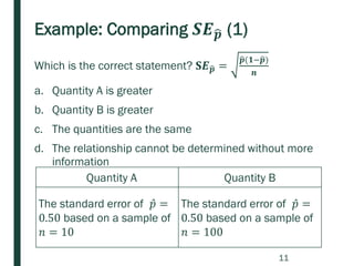
Example: Comparing 𝑺𝑬ෝ𝒑 (1)
Which is the correct statement? 𝐒𝑬ෝ𝒑 =
ෝ𝒑(𝟏−ෝ𝒑)
𝒏
a. Quantity A is greater
b. Quantity B is greater
c. The quantities are the same
d. The relationship cannot be determined without more
information
Quantity A Quantity B
The standard error of Ƹ𝑝 =
0.50 based on a sample of
𝑛 = 10
𝑛 = 100
11

𝒏
information
𝑛 = 10
𝑛 = 100
12

TOP HAT Which is the correct statement? 𝐒𝑬ෝ𝒑 =
𝒏
information
The standard error
of Ƹ𝑝 = 0.50 based on a
sample of 𝑛 = 10
𝑛 = 10
13

MAKE UP Which is the correct statement? 𝐒𝑬ෝ𝒑 =
𝒏
information
The standard error of
Ƹ𝑝 = 0.05 based on a
sample of 𝑛 = 10
The standard error of
Ƹ𝑝 = 0.95 based on a
sample of 𝑛 = 10
14

TOP HAT Which is the correct statement? 𝐒𝑬ෝ𝒑 =
𝒏
information
The standard error
of Ƹ𝑝 = 0.60
0.45
15

Confidence Intervals for a single population
proportion
16
■ The sample proportion ෝ𝒑 provides our best guess, called
a point estimate, for the value of the population
proportion 𝑝, but it is not 100% accurate.
■ Recall the general format for a confidence interval
estimate is given by:
Point estimate ± (a few) standard errors
“a few” depends on how confident we want to be that our
interval contains the true parameter.

Confidence interval for population proportion
This goes in the box on Page 100
■ An approximate Y% confidence interval (CI) for the population
proportion p is:
ෝ𝒑 ± 𝒛∗ ෝ𝒑(𝟏−ෝ𝒑)
𝒏
■ The margin of error is:
𝒛∗
ෝ𝒑(𝟏 − ෝ𝒑)
𝒏
■ z* is determined by the confidence level, Y.
Given a confidence interval (a, b)
■ The mid-point of the confidence interval is ෝ𝒑 =
𝒃+𝒂
𝟐
■ The width is two times the margin of error. Or, the margin of error is
half the width, 𝑴𝑬 =
𝒃−𝒂
𝟐
17

Example: What is the ideal family size? (1)
In 2018 a random sample of 1,017 American adults was
asked the question, “What do you think is the ideal number
of children for a family to have?” Results showed that 41%
of respondents said three or more children is ideal.
a. Use the reported percentage and sample size to check
the expected success/failure condition for a confidence
interval.
18

Expected success/failure check
Pay attention to notation!
■ For Confidence Intervals:
– Check to see if 𝑛 Ƹ𝑝 ≥ 10 𝑎𝑛𝑑 𝑛 1 − Ƹ𝑝 ≥ 10.
– Here we use the sample proportion, Ƹ𝑝.
■ For Hypothesis Tests
– Check to see if 𝑛𝑝0 ≥ 10 𝑎𝑛𝑑 𝑛(1 − 𝑝0) ≥ 10.
– Here we use the null value, 𝑝0.
19

In 2018 a random sample of 1,017 American adults was
asked the question, “What do you think is the ideal number
of children for a family to have?” Results showed that 41%
of respondents said three or more children is ideal.
a. Use the reported percentage and sample size to check
the expected success/failure condition for a confidence
interval.
■ 1017 x 0.41 = 416.97, clearly at least 10
■ 1017 x (1 – 0.41) = 600.03, clearly at least 10
■ To find a 90% CI what multiplier should we use? TOP HAT
20

b. Calculate a 90% confidence interval for the proportion of
Americans who think that three or more children is the ideal
family size, and interpret the interval in context.
WARNING: Do not round numbers during calculation.
ෝ𝒑 ± 𝒛∗ ෝ𝒑(𝟏−ෝ𝒑)
𝒏
= 𝟎. 𝟒𝟏 ± 𝟏. 𝟔𝟒𝟒𝟖𝟓𝟑𝟔 ×
𝟎.𝟒𝟏×𝟎.𝟓𝟗
𝟏𝟎𝟏𝟕
So, a 90% CI for p is given by (0.3846, 0.4354)
c. A 95% confidence interval produced from the same survey
results would be
narrower wider the same width as
the interval computed in (b). TOP HAT
21

Choosing a sample size when estimating
We are on PAGE 102. We will come back to 101 later.
■ Many times, once we have calculated a confidence interval for
a population parameter, we find that the interval is too wide to
be useful. In such a case we would like to reduce the margin
of error.
■ Recall that the margin of error for a confidence interval is
𝑀𝐸 = 𝑧∗
∙ 𝑆𝐸
■ To reduce the size of the margin of error we have two choices:
1. reduce the confidence level
2. decrease the SE by increasing the sample size
22

Costs and benefits
■ Both options have their costs and benefits.
■ Narrower intervals are more desirable because they give us
more precision in our estimates.
■ Reducing the confidence level from say, 95% to 90% will give
us a narrower interval but will also increase our uncertainty
about whether the parameter is in our interval.
■ Increasing the sample size can narrow the interval without
increasing uncertainty, but it involves extra financial costs to
collect more data.
23

Solving for n
■ The margin of error for confidence intervals for a single
proportion is
𝑀𝐸 = 𝑧∗
𝑝 1 − 𝑝
𝑛
■ Solving this formula for 𝑛 gives us
𝑀𝐸2 = (𝑧∗)2
𝑝(1 − 𝑝)
𝑛
𝑛 = 𝑝(1 − 𝑝)
𝑧∗
𝑀𝐸
2
24

Planning value for p
■ If we have a value from a previous or similar sample, we
will use that as a planning value, 𝒑∗.
■ What to do if we do not have a planning value from a
previous sample?
■ We need to plug in some value for p* right?
■ What value should we use?
■ Recall, Comparing SE (2)
25

𝒏
TOP HAT
information
The standard error
of Ƹ𝑝 = 0.50 based on a
sample of 𝑛 = 10
𝑛 = 10
26

Planning value for p
■ If we have a value from a previous or similar sample, we will use that
as a planning value, 𝒑∗.
■ What to do if we do not have
a planning value from a previous
sample?
■ On the graph, the y values
are p(1 - p).
■ Notice the maximum occurs
at p = 0.5
■ The margin of error 𝑀𝐸 = 𝑧∗ 𝑝 1−𝑝
𝑛
for a proportion (as well as the
SE) is largest when 𝑝 = 0.5, so as a worst case scenario we will use
𝑝∗
= 0.5 if no better estimate of the planning value is available.
■ Since we cannot have a non-integer value for n (for example you
can’t sample 621.25 people!), we will ALWAYS ALWAYS ALWAYS
ROUND UP to the next whole number.
27
y = p(1 –p)

WHY DO WE ALWAYS ROUND UP?
■ The margin of error for confidence intervals for a single
proportion is
𝑀𝐸 ≥ 𝑧∗
𝑝 1 − 𝑝
𝑛
■ Solving this formula for 𝑛 gives us
𝑀𝐸2 ≥ (𝑧∗)2
𝑝(1 − 𝑝)
𝑛
𝑛 ≥ 𝑝(1 − 𝑝)
𝑧∗
𝑀𝐸
2
■ This is why, we have to always round up!!!
28

Charity care (1)
Suppose a preliminary simple random sample of 75 physicians in
Michigan showed that 42 provided at least some charity care
(i.e., treated poor people at no cost). We want to estimate the
proportion of all physicians in Michigan who provide some charity
care with 90% confidence.
a. If you want the 90% confidence interval to have a margin of
error of no more than 2.5%, what is the minimum sample size
you should take? Use the information from the preliminary
sample as a planning value, 𝑝∗.
■ Note the following:
■ Planning value: p*=42/75 =0.56, keep all decimal places
■ Multiplier: z*=1.64486, keep more decimal places
■ ME= 0.025, must change to a decimal, don’t use %
𝒏 = 𝒑 𝟏 − 𝒑
𝒛∗
𝑴𝑬
𝟐
= 𝟎. 𝟓𝟔(𝟏 − 𝟎. 𝟓𝟔)(
𝟏.𝟔𝟒𝟒𝟖𝟔
𝟎.𝟎𝟐𝟓
) 𝟐
=1066.64
■ So, ROUND UP TO GET the required sample size to be 1067.
29

Charity care (2)
b. Suppose you had no preliminary information about the proportion of
physicians who provide some charity care, but still want the 90% confidence
interval to have a margin of error of no more than 2.5%. What is the
minimum sample size we need?
■ Note the following:
■ Planning value: p*=0.5, worst estimate
■ Multiplier: z*=1.64486, keep more decimal places
■ ME= 0.025, must change to a decimal, don’t use %
𝒏 = 𝒑 𝟏 − 𝒑
𝒛∗
𝑴𝑬
𝟐
= 𝟎. 𝟓(𝟏 − 𝟎. 𝟓)(
𝟏.𝟔𝟒𝟒𝟖𝟔
𝟎.𝟎𝟐𝟓
) 𝟐
=1082.22
Why is it better to use a pilot sample where possible?
■ The planning value p* =0.5 is the worst.
■ It makes the ME largest, so less precision.
■ It also increases the sample size required, so more cost in terms of
collecting a large sample.
30

Review question
c. Suppose a new, larger sample of physicians is selected and we
calculate a standard error for the sample proportion to be 1.52%.
What is the correct interpretation of this standard error?
i. In repeated samples of this size, we expect the sample
proportion to be within 1.52% of the true population
proportion, on average.
ii. The margin of error for the new confidence interval is
1.52%.
iii. If we take repeated samples, 90% of the sample
proportions will be within 1.52% of the upper and lower
bounds of our calculated confidence interval.
iv. Our confidence interval will include the true population
proportion 1.52% of the time.
31

Review question
c. Suppose a new, larger sample of physicians is selected and we
calculate a standard error for the sample proportion to be 1.52%.
What is the correct interpretation of this standard error?
i. In repeated samples of this size, we expect the sample
proportion to be within 1.52% of the true population
proportion, on average.
ii. The margin of error for the new confidence interval is
1.52%.
iii. If we take repeated samples, 90% of the sample
proportions will be within 1.52% of the upper and lower
bounds of our calculated confidence interval.
iv. Our confidence interval will include the true population
proportion 1.52% of the time.
32

Hypothesis tests for a single proportion
Recall the Basic Steps in Any Hypothesis Test
1. Determine appropriate null and alternative
hypotheses.
2. Check assumptions for performing the test.
3. Calculate the test statistic and determine the p-
value.
4. Evaluate the p-value and the compatibility of the
null model.
5. If necessary, make a recommendation in the
context of the problem.
33

Hypothesis tests for a single proportion
We will from now on write the hypothesis in
terms of Parameters when possible.
In the context of testing about the value of a
population proportion p, the possible
hypotheses statements are:
■ H0: 𝒑 = 𝒑 𝟎 versus Ha: 𝒑 ≠ 𝒑 𝟎
■ H0: 𝒑 = 𝒑 𝟎 versus Ha: 𝒑 < 𝒑 𝟎
■ H0: 𝒑 = 𝒑 𝟎 versus Ha: 𝒑 > 𝒑 𝟎
34

What is this 𝒑 𝟎?
■ Where does p0 come from?
■ This is the hypothesized value of the population
proportion 𝒑 that the null hypothesis believes to be true.
■ Our test uses the normal model 𝑁(𝑝, 𝑆𝐸ො𝑝),
where 𝑆𝐸ො𝑝 =
𝑝 1−𝑝
𝑛
.
■ Problematically, we don’t know the value of 𝑝, and so
need to use a substitute.
KEY IDEA: To conduct the hypothesis test, we assume that
the null hypothesis is true, that is, we take the population
proportion p = p0 to build the null model using Normal
distribution and Central Limit Theorem.
35

How do we find p-value?
■ So the standardized test statistic, z-statistic for a sample
proportion in testing is:
z =
𝒐𝒃𝒔𝒆𝒓𝒗𝒆𝒅−𝒆𝒙𝒑𝒆𝒄𝒕𝒆𝒅
𝒏𝒖𝒍𝒍 𝒔𝒕𝒂𝒏𝒅𝒂𝒓𝒅 𝒆𝒓𝒓𝒐𝒓
=
ෝ𝒑−𝒑 𝟎
𝒑 𝟎 𝟏−𝒑 𝟎
𝒏
■ Under the null model, this z-test statistic will have
approximately a Standard Normal distribution Z ~ N(0, 1)
■ The standard normal distribution Z will be used to
compute the p-value for the test.
36

Example: Left-handed artists
■ About 10% of the human population is left-handed.
■ Suppose that a researcher speculates that artists are
more likely to be left-handed than are other people in the
general population.
■ The researcher surveys a random sample of 150 artists
and finds that 18 of them are left-handed.
■ Let us perform the test following the steps to test the
researcher’s claim.
37

Step 1: Determine the appropriate null and alternative
hypotheses.
First let us write down the hypothesis in terms of the
parameter, population proportion p.
■ H0: 𝒑 = 𝟎. 𝟏𝟎 Ha: 𝒑 > 𝟎. 𝟏𝟎
where the parameter p represents
the population proportion of artists who are left handed
■ Note: The direction of extreme is right-tailed based on
the ALTERNATIVE HYPOTHESIS.
38

Step 2: Check the success-failure assumption for
performing the test.
Condition 1: The data are assumed to be a random sample.
Condition 2: Check if np0  10 and n(1 – p0)  10.
39

Expected success/failure check
Pay attention to notation!
■ For Hypothesis Tests
– Check to see if 𝑛𝑝0 ≥ 10 𝑎𝑛𝑑 𝑛(1 − 𝑝0) ≥ 10.
– Here we use the null value, 𝑝0.
40

Condition 1: The data are assumed to be a random sample.
■ 150 x 0.1 = 15, Note here we use the null value of 0.1
and not the sample proportion 18/150
■ 150 x (1 - 0.1)= 150 x 0.9 = 135.
■ Both, the expected successes and expected failures are
at least 10.
Is it appropriate to use a normal model for this test?
■ Yes, both the independence and expected
success/failure conditions are satisfied.
41

Step 3: Calculate the test statistic
Observed test statistic:
𝑧 =
Ƹ𝑝 − 𝑝0
𝑝0 1 − 𝑝0
𝑛
=
18
150
− 0.1
0.1(1 − 0.1)
150
Note: We use the null value 0.1 in the denominator for the
standard error calculation and not the sample proportion
18/150.
Plug and chug to get, z = 0.816496
42

Step 3: Determine the p-value.
Recall:
The p-value is the probability of getting a test statistic as
extreme or more extreme than the observed test statistic
value, under the null model. Since we have a one-sided test
to the right, toward the larger values …
p-value = probability of getting a z test statistic as large or
larger than the observed z test statistic, assuming the null
hypothesis is true.
43

Step 3: Calculate the test statistic and determine the p-
value.
■ Test statistic is z=0.816496
■ p-value = ?
■ What function in GC?
■ normalcdf
■ Lower= 0.816496
■ Upper= 1010
■ Mean = 0
■ SD = 1
■ p-value = 0.2071
44

Step 4: Evaluate the p-value and the compatibility of the null
model with observed results.
■ p-value = 0.2071 is greater than 0.10, so there is LITTLE
EVIDENCE to say that the null model IS NOT compatible
with the observed results.
■ In the context of the question, there is little evidence to
say that the proportion of artists who are left-handed is
greater than 10%
45

Example: Getting along with parents (1)
In a Gallup Youth Survey n = 501 randomly selected
American teenagers were asked about how well they get
along with their parents. One survey result was that 54% of
the sample said they get along “VERY WELL” with their
parents.
a) The sample proportion was found to be 0.54. Check the
expected success/failure condition.
■ 501 x 0.54 is more than 10
■ 501 x 0.46 is also more than 10
46

b) Find the standard error for the sample proportion and
use it to complete the sentence in part c that interprets
the standard error in terms of an average distance.
𝐒𝑬ෝ𝒑 =
𝒏
=TOP HAT
c) We would estimate the average distance between the
possible _ _ values (from repeated samples) and
_ ____ to be about _________.
47

b) Find the standard error for the sample proportion and
use it to complete the sentence in part c that interprets
the standard error in terms of an average distance.
𝐒𝑬ෝ𝒑 =
𝒏
=
𝟎. 𝟓𝟒 × 𝟎. 𝟒𝟔
𝟓𝟎𝟏
= 𝟎. 𝟎𝟐𝟐𝟐𝟔𝟔𝟕
c) We would estimate the average distance between the
possible ___ෝ𝒑___ values (from repeated samples) and
_ the population proportion p____ to be about
___0.0223______.
48

d) Compute a 95% confidence interval for the population
proportion of teenagers that get along very well with
their parents.
■ 95% CI for p:
ෝ𝒑 ± 𝒛∗
𝒏
𝑻𝑶𝑷 𝑯𝑨𝑻
49

d) Compute a 95% confidence interval for the population
proportion of teenagers that get along very well with
their parents.
■ 95% CI for p:
ෝ𝒑 ± 𝒛∗
𝒏
= ( ෝ𝒑 − 𝒛∗ ෝ𝒑 𝟏−ෝ𝒑
𝒏
, ෝ𝒑 + 𝒛∗ ෝ𝒑 𝟏−ෝ𝒑
𝒏
)
= ( 𝟎. 𝟓𝟒 − 𝟏. 𝟗𝟔 ×
𝟎.𝟓𝟒×𝟎.𝟒𝟔
𝟓𝟎𝟏
, 𝟎. 𝟓𝟒 + 𝟏. 𝟗𝟔 ×
𝟎.𝟓𝟒×𝟎.𝟒𝟔
𝟓𝟎𝟏
)
= (𝟎. 𝟒𝟗𝟔𝟒, 𝟎. 𝟓𝟖𝟑𝟔)
50

e) Fill in the blanks for the typical interpretation of the
confidence interval in part c:
“Based on this sample, with 95% confidence, we would
estimate that somewhere between __49.64%___ and
__58.36%_ of all American teenagers think they get along
very well with their parents.”
f) Can we say that 95% of the time the population
proportion p will be in above (already observed) interval
you computed in part (c)?
■ TOP HAT
51

e) Fill in the blanks for the typical interpretation of the
confidence interval in part c:
“Based on this sample, with 95% confidence, we would
estimate that somewhere between __49.64%___ and
__58.36%_ of all American teenagers think they get along
very well with their parents.”
f) Can we say that 95% of the time the population
proportion p will be in above (already observed) interval
you computed in part (c)?
■ NO, remember Harry Potter 1. The population proportion
p is a fixed value. After we construct the interval, p is
either inside surely or not inside surely. We cannot tell
unless we know the true value of p.
52

Getting along with parents again
■ Recall the 95% confidence interval for the true
proportion of American teenagers who say they get along
“very well” with their parents gave us the result
Ƹ𝑝 ± 𝑧∗
Ƹ𝑝(1 − Ƹ𝑝)
𝑛
= 0.54 ± 1.96
0.54(1 − 0.54)
501
■ What is the margin of error?
■ The margin of error is
𝑧∗ ො𝑝(1− ො𝑝)
𝑛
= 1.96
0.54(1−0.54)
501
= 0.0436, meaning that our
margin of error is about 4.4% points.
53

Smaller ME at 95% confidence level
■ Suppose we want a margin of error less than 0.03? What
size sample should we take?
■ Planning value: p*=0.54 and Multiplier: z*=1.96
■ ME= 0.03,
■ 𝒏 = 𝒑 𝟏 − 𝒑
𝒛∗
𝑴𝑬
𝟐
= 𝟎. 𝟓𝟒(𝟏 − 𝟎. 𝟓𝟒)(
𝟏.𝟗𝟔
𝟎.𝟎𝟑
) 𝟐=1060.28
■ So, ROUND UP TO GET the required sample size to be
1061.
■ Calculate the sample size needed for a margin of error
less than 0.01.
■ TOP HAT
54

Smaller ME at 95% confidence level
■ Suppose we want a margin of error less than 0.03? What size
sample should we take?
■ Planning value: p*=0.54 and Multiplier: z*=1.96
■ ME= 0.03,
■ 𝒏 = 𝒑 𝟏 − 𝒑
𝒛∗
𝑴𝑬
𝟐
= 𝟎. 𝟓𝟒(𝟏 − 𝟎. 𝟓𝟒)(
𝟏.𝟗𝟔
𝟎.𝟎𝟑
) 𝟐
=1060.28
■ Calculate the sample size needed for a margin of error less
than 0.01.
■ 𝒏 = 𝒑 𝟏 − 𝒑
𝒛∗
𝑴𝑬
𝟐
= 𝟎. 𝟓𝟒(𝟏 − 𝟎. 𝟓𝟒)(
𝟏.𝟗𝟔
𝟎.𝟎𝟏
) 𝟐
=9542.53
■ So, round up to get the required sample size to be 9543.
55

Example: Households without Children
The US Census reports that 48% of households have no
children. A Random Sample of 500 Households was taken
to assess if the population proportion has changed from
0.48. Of the 500 households, 220 had no children.
Step 1: Determine the appropriate null and alternative
hypotheses.
H0: p = 0.48 Ha: p ≠ 0.48
where the parameter p represents the population
proportion of all households today that have no children.
Note: The direction of extreme is two-sided.
56

Condition 1: The data is assumed to come from a random
sample.
■ Don’t use 220/500 to check conditions!!!
■ 500x0.48 and 500x0.52 are both more than 10
Is it appropriate to use a normal model for this test?
Yes, both conditions are satisfied.
57

Step 3: Calculate the test statistic and determine the p-
value.
𝑧 =
Ƹ𝑝 − 𝑝0
𝑝0 1 − 𝑝0
𝑛
=
220
500
− 0.48
0.48 × 0.52
500
= −1.7903
58

Step 3: Calculate the test statistic and determine the p-value.
■ The p-value is the probability of getting a test statistic as extreme or
more extreme than the observed test statistic value, using the null
hypothesis model.
■ Since we have
a two-tailed test,
both large and small
values are “extreme”.
■ p-value= 0.0734
Answer:
2 x normalcdf
Lower -1010
Upper −1.7903
Mean 0
SD 1
59

Step 4: Evaluate the p-value and the compatibility of the null
model with observed results.
■ p-value= 0.0734 is between 0.05 and 0.10.
■ So, some evidence to say that the null model is not
compatible with our data.
■ Some evidence based on the sample data to say that the
proportion of households without children is different
from 48%.
60

3.2 Inference for 𝒑 𝟏 − 𝒑 𝟐, a difference in
population proportions
Applying the sampling distribution for Ƹ𝑝1 − Ƹ𝑝2:
1. Random samples are taken separately from two
populations and the same categorical response variable
is recorded for each individual.
2. One random sample is taken from a single
homogeneous population and a categorical variable is
recorded for each individual, but then units are
categorized as having one characteristic or another, e.g.
old/young.
3. Participants are randomly assigned to one of two
treatment conditions, and the same categorical
response variable, such as weight loss status, is
recorded for each individual unit.
61

Sampling Distribution of ො𝑝1 − ො𝑝2
THIS SLIDE HAS BEEN MODIFIED SLIGHTLY
KEY IDEA: If the following conditions are met, the sampling
distribution of Ƹ𝑝1 − Ƹ𝑝2 will be approximately normal .
■ Condition #1: For each sample, the sample proportion’s
distribution can be modeled by a normal distribution.
That is, in each sample, the observations are independent
of each other and for each sample, the success/failure
condition is met.
■ Condition #2: The two samples are independent of one
another.
62

Sampling Distribution of ො𝑝1 − ො𝑝2
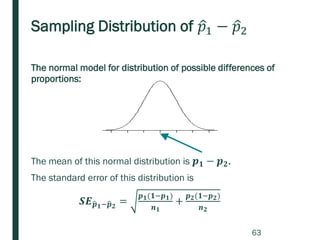
The normal model for distribution of possible differences of
proportions:
The mean of this normal distribution is 𝒑 𝟏 − 𝒑 𝟐.
The standard error of this distribution is
𝑺𝑬ෝ𝒑 𝟏−ෝ𝒑 𝟐
=
𝒑 𝟏(𝟏−𝒑 𝟏)
𝒏 𝟏
+
𝒑 𝟐(𝟏−𝒑 𝟐)
𝒏 𝟐
63

Checking success/failure condition
■ The approximate normal model for the sampling
distribution of the difference in sample proportions
requires that the quantities
■ 𝑛1 𝑝1, 𝑛1(1 − 𝑝1), 𝑛2 𝑝2, and 𝑛2(1 − 𝑝2) are at least 10.
■ Since the population proportions are unknown, we will
check if the condition is met using the sample estimates.
■ For confidence interval estimation we will need that the
quantities 𝑛1 Ƹ𝑝1, 𝑛1(1 − Ƹ𝑝1), 𝑛2 Ƹ𝑝2, and 𝑛2(1 − Ƹ𝑝2) are all
at least 10.
■ For hypothesis testing, we will replace the population
proportions with an appropriate estimate under the null
hypothesis assumption that the proportions are equal, so
watch for that subtle difference in checking the expected
success/failure condition.
64

Expected success/failure condition
■ For confidence intervals:
■ Use sample proportions, Ƹ𝑝1 𝑎𝑛𝑑 Ƹ𝑝2
𝑛1 Ƹ𝑝1, 𝑛1(1 − Ƹ𝑝1), 𝑛2 Ƹ𝑝2, 𝑛2(1 − Ƹ𝑝2) are all at least 10.
■ For hypothesis testing:
■ Use the pooled estimate, ෝ𝒑
𝑛1 Ƹ𝑝, 𝑛1(1 − Ƹ𝑝), 𝑛2 Ƹ𝑝, 𝑛2(1 − Ƹ𝑝) are all at least 10.
65

Confidence Intervals for 𝑝1 − 𝑝2
■ After checking conditions, we can use the following
formula to calculate a confidence interval for 𝑝1 − 𝑝2:
𝑃𝑜𝑖𝑛𝑡 𝑒𝑠𝑡𝑖𝑚𝑎𝑡𝑒 ± 𝑧∗ × 𝑆. 𝐸.
Ƹ𝑝1 − Ƹ𝑝2 ± 𝑧∗
Ƹ𝑝1 1 − Ƹ𝑝1
𝑛1
+
Ƹ𝑝2 1 − Ƹ𝑝2
𝑛2
■ Alternatively, we can use the Graphic Calculator function
2propZint
66

Example: Market research
■ Companies spend hundreds of billions of dollars in
advertising every year.
■ Suppose an advertising company is conducting research
to evaluate the effectiveness of a client’s new advertising
campaign.
■ Before the new campaign begins, a telephone survey of
550 households in the test market area showed 68
households are “aware” of the client’s product.
■ The new campaign is then initiated with TV, radio, and
newspaper advertisements running for three weeks.
■ A survey conducted immediately after the new campaign
showed 151 of 700 households are “aware” of the
client’s product.
67

a. Compute the 90% confidence interval for the difference in the
proportion of households before and after the campaign who
are “aware” of the client’s product.
90% CI for 𝒑 𝒂𝒇𝒕𝒆𝒓 − 𝒑 𝒃𝒆𝒇𝒐𝒓𝒆:
In Graphic Calculator,
Subscripts: 1 = after and 2 = before
2propZint
𝒙 𝟏 = 𝟏𝟓𝟏
𝒏 𝟏 = 𝟕𝟎𝟎
𝒙 𝟐 = 𝟔𝟖
𝒏 𝟐 = 𝟓𝟓𝟎
Clevel= 0.90
Answer: (0.05763, 0.12653)
68

b. How do we interpret this interval?
■ We are 90% confident (in the procedure) that the true
difference in proportions of households after and before the
ad campaign who are aware of the client’s product is between
0.05763 (5.763%) and 0.12653(12.653%).
c. How do we interpret the level of this interval?
■ Amount of confidence in the procedure!
■ If repeated samples of the same sizes are collected and we
construct 90% CI using each one of the sample results, then
we expect 90% of those intervals to contain the true
difference in proportions of households after and before the
ad campaign who are aware of the client’s product.
69

Hypothesis testing when 𝑯 𝟎: 𝒑 𝟏 = 𝒑 𝟐
■ Often, we are interested in assessing whether there is a
difference in the rate or proportion of a certain
categorical variable across two independent (parts of
populations or) populations.
■ Just as with confidence intervals, we’ll apply a normal
model to the sampling distribution of Ƹ𝑝1 − Ƹ𝑝2 to conduct
our hypothesis test.
70

Example: Stomach pains
■ In a randomized, controlled double-blind study of a new
drug, there were 357 people in the treatment group and
285 in the control group.
■ It was found that 155 people in the treatment group
experienced stomach pains, whereas 98 people in the
control group experienced stomach pains.
■ It’s helpful to organize the information using a table:
Group Stomach
pain
No
stomach
pain
Total
Treatment 155 202 357 Ƹ𝑝𝑡𝑟𝑒𝑎𝑡𝑚𝑒𝑛𝑡 = 𝟎. 𝟒𝟑𝟒𝟐
Control 98 187 285 Ƹ𝑝 𝑐𝑜𝑛𝑡𝑟𝑜𝑙 = 𝟎. 𝟑𝟒𝟑𝟗
71

Example: Stomach pains
■ What is the research question?
■ Does the drug have a greater rate of stomach pain than the
placebo?
■ Set up the appropriate hypotheses to test for an investigation
as to whether there is an increased rate of stomach pains in
the treatment group.
■ Let 𝑝1 represent the proportion of patients in the treatment
group with stomach pain
■ Let 𝑝2 represent the proportion of patients in the control group
with stomach pain
■ 𝐻0: 𝑝1 = 𝑝2
■ 𝐻 𝑎: 𝑝1 > 𝑝2 Note: Right-tailed alternative!
■ Note in the case of Hypothesis testing the center for the
normal approximation will be 0.
72

Computing the standard error 𝑆𝐸ො𝑝1− ො𝑝2
in
hypothesis tests
■ In general, standard error for Ƹ𝑝𝑡𝑟𝑒𝑎𝑡𝑚𝑒𝑛𝑡 − Ƹ𝑝 𝑐𝑜𝑛𝑡𝑟𝑜𝑙 would
be
𝑆𝐸ො𝑝1− ො𝑝2
=
𝑝1 1 − 𝑝1
𝑛1
+
𝑝2 1 − 𝑝2
𝑛2
■ But under the null hypothesis, 𝑝1 = 𝑝2, so if we call that
value p, we have the null standard error
𝑆𝐸ො𝑝1− ො𝑝2
=
𝑝 1 − 𝑝
𝑛1
+
𝑝 1 − 𝑝
𝑛2
= 𝑝(1 − 𝑝)(
1
𝑛1
+
1
𝑛2
)
73

Pooled estimate of p
■ Problematically, we don’t know the common rate of
stomach pains, 𝑝, but we can obtain a good estimate of
it by pooling the results of both samples.
Ƹ𝑝 =
𝑥1 + 𝑥2
𝑛1 + 𝑛2
■ What are 𝑥1 𝑎𝑛𝑑 𝑥2? How to find them?
■ TOP HAT
74

Pooled estimate of p
■ Problematically, we don’t know the common rate of
stomach pains, 𝑝, but we can obtain a good estimate of
it by pooling the results of both samples.
Ƹ𝑝 =
# 𝑜𝑓 ′𝑠𝑢𝑐𝑐𝑒𝑠𝑠𝑒𝑠′
# 𝑜𝑓 𝑐𝑎𝑠𝑒𝑠
=
𝑥1 + 𝑥2
𝑛1 + 𝑛2
■ This is called the pooled estimate of the sample
proportion under the assumption the null is true.
■ We use it to compute the null standard error and to verify
the expected success/failure condition.
75

Expected success/failure condition
■ For confidence intervals:
■ Use sample proportions, Ƹ𝑝1 𝑎𝑛𝑑 Ƹ𝑝2
𝑛1 Ƹ𝑝1, 𝑛1(1 − Ƹ𝑝1), 𝑛2 Ƹ𝑝2, 𝑛2(1 − Ƹ𝑝2) are all at least 10.
■ For hypothesis testing:
■ Use the pooled estimate, ෝ𝒑
𝑛1 Ƹ𝑝, 𝑛1(1 − Ƹ𝑝), 𝑛2 Ƹ𝑝, 𝑛2(1 − Ƹ𝑝) are all at least 10.
76

Stomach pains
Group Stomach
pain
No
stomach
pain
Total Ƹ𝑝
Treatment 155 202 357 0.4342
Control 98 184 285 0.3123
a. Calculate the pooled proportion Ƹ𝑝 and use it to check the
estimated success/failure condition for performing the test.
Ƹ𝑝 =
# 𝑜𝑓 ′𝑠𝑢𝑐𝑐𝑒𝑠𝑠𝑒𝑠′
# 𝑜𝑓 𝑐𝑎𝑠𝑒𝑠
=
𝑥1 + 𝑥2
𝑛1 + 𝑛2
=
155 + 98
357 + 285
= 0.394
■ Check if each one below is at least 10:
357 × 0.394 357 × (1 − 0.394)
285 × 0.394 285 × (1 − 0.394)
■ This is a randomized, controlled double-blind study. So, we
can assume that the samples are independent and that the
observations in each sample are also independent.
77

Stomach pains
b. Calculate the test statistic.
𝑧 =
ො𝑝1− ො𝑝2
𝑆𝐸ෝ𝑝1−ෝ𝑝2
where 𝑆𝐸ො𝑝1− ො𝑝2
= 𝑝(1 − 𝑝)(
1
𝑛1
+
1
𝑛2
)
Using Ƹ𝑝 = 0.394, 𝑆𝐸ො𝑝1− ො𝑝2
= 0.394 1 − 0.394
1
357
+
1
285
𝒛 =
ෝ𝒑 𝟏−ෝ𝒑 𝟐
𝑺𝑬ෝ𝒑 𝟏−ෝ𝒑 𝟐
=
𝟏𝟓𝟓
𝟑𝟓𝟕
−
𝟗𝟖
𝟐𝟖𝟓
𝟎.𝟎𝟑𝟖𝟖𝟏𝟓
= 𝟐. 𝟑𝟐𝟔𝟖
c. Sketch and calculate the p-value.
P-value= 0.01, right-tail.
Check using 2propZtest in GC!
78

Stomach pains
d. Evaluate the reasonableness of the null model.
■ P-value is 0.01, so very strong
evidence to say that the null model
is not compatible with the sample data.
■ That is, very strong evidence to say
that the proportion of patients with
stomach pain in the treatment group
is greater than the proportion of
patients with stomach pain in the
control group.
79

Example: Taking More Pictures with Cell
■ A study found that more than 75% of young adults use their
cell phones for taking pictures at least 2 times per week and
suggested that the proportion for young women is higher than
for young men.
■ A follow-up study was conducted to investigate this conjecture.
■ H0: 𝑝1 = 𝑝2 versus Ha: 𝑝1 > 𝑝2
■ p1 represents the population proportion of all young women
18-25 years old who report using their cell phone to take
pictures at least 2 times per week, and
■ p2 represents the population proportion of all young men 18-
25 years old who report using their cell phone to take pictures
at least 2 times per week.
80

Age group = 18 – 25 year olds
Young
Women
Young
Men
Number who report using phone to take pictures at
least 2 times/week
417 369
Sample Size 521 492
Percent 80% 75%
Results:
■ We can assume these samples are independent random
samples.
■ Verify the remaining assumption necessary to conduct
the Z test.
■ What is the remaining assumption?
■ TOP HAT
81

Let us conduct the test.
■ Calculate the test-statistic and p-value.
■ TOP HAT x 2
■ Calculate the observed difference in sample proportions of
young women and young men
■ 0.80 - 0.75 = 0.05 (5%)
Age group = 18 – 25 year olds
Young
Women
Young
Men
Number who report using phone to take pictures at
least 2 times/week
417 369
Sample Size 521 492
Percent 80% 75%
82

■ Consider each of the following conclusions. Which among them is
the least appropriate interpretation of the test results?
■ TOP HAT
a. We interpret the test results to mean that the population proportion
of all young women 18-25 years old who take pictures with their
phone at least twice per week is about 5 percent higher than that of
the population of all young men 18-25 years old.
b. There is strong evidence a person’s gender influenced the rate at
which they adopted the use of cell phones as cameras. Marketing
firms should adapt their advertising plans to account for the
findings that young adult women use cell phones in a manner
different than their male counterparts.
c. There is strong evidence a person’s gender influenced the rate at
which they adopted the use of cell phones as cameras. Marketing
firms might consider conducting more research to determine just
how large the effect detected by this study might be.
83

Chapter 3

More Related Content

What's hot

Similar to Chapter 3

More from EasyStudy3

Recently uploaded

Chapter 3