The document discusses several information retrieval models including the Boolean, vector space, and probabilistic models. It provides details on how each model represents documents and queries, defines relevance, and ranks documents in response to queries. Specifically, it describes: 1) The Boolean model uses exact matching to retrieve only documents that satisfy a Boolean query, but does not rank results. 2) The vector space model represents documents and queries as vectors of term weights and ranks documents based on their similarity to the query vector using measures like cosine similarity. 3) Term frequency-inverse document frequency (TF-IDF) is discussed as a method to weight terms based on their importance.

1. UNIT III
MODELING AND RETRIEVAL EVALUATION
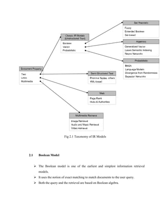
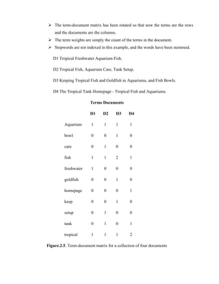
2. Basic Retrieval Models
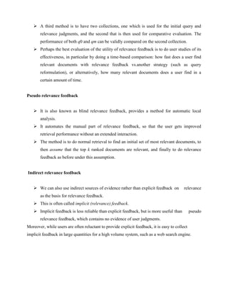
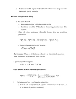
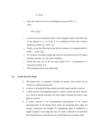
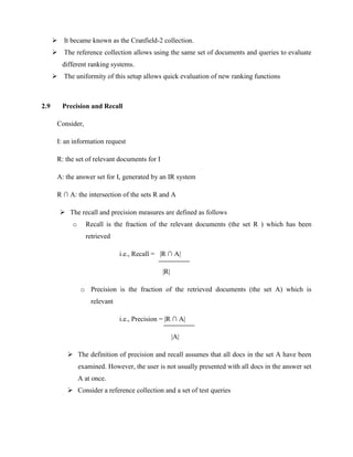
 An IR model governs how a document and a query are represented and how the relevance
of a document to a user query is defined.
 There are Three main IR models:
 Boolean model
 Vector space model
 Probabilistic model
 Although these models represent documents and queries differently, they used the same
framework. They all treat each document or query as a “bag” of words or terms.
 Term sequence and position in a sentence or a document are ignored. That is, a document
is described by a set of distinctive terms.
 Each term is associated with a weight.Given a collection of documents D, let
V = {t1, t2... t|V|} be the set of distinctive terms in the collection, where ti is a term.
 The set V is usually called the vocabulary of the collection, and |V| is its size,
i.e., the number of terms in V.
 A weight wij > 0 is associated with each term ti of a document dj D. A weight wij > 0
is associated with each term ti of a document dj D.For a term that does not appear in
document dj, wij = 0.
 Each document dj is thus represented with a term vector, dj = (w1j, w2j, ..., w|V|j),where
each weight wij corresponds to the term ti V, and quantifies the level of importance of ti
in document dj.
An IR model is a quadruple [D, Q, F, R(qi, dj)] where
1. D is a set of logical views for the documents in the collection
2. Q is a set of logical views for the user queries
3. F is a framework for modeling documents and queries
4. R(qi, dj) is a ranking function

2. Fig 2.1 Taxonomy of IR Models
2.1 Boolean Model
 The Boolean model is one of the earliest and simplest information retrieval
models.
 It uses the notion of exact matching to match documents to the user query.
 Both the query and the retrieval are based on Boolean algebra.

3. Document Representation:
 In the Boolean model, documents and queries are represented as sets of terms.
 That is, each term is only considered present or absent in a document.
 Using the vector representation of the document above, the weight wij ( {0, 1})
of term ti in document dj is 1 if ti appears in document dj, and 0 otherwise, i.e.,
Wij = 1 if appears in dj
0 otherwise.
Boolean Queries:
 Query terms are combined logically using the Boolean operators AND, OR, and
NOT, which have their usual semantics in logic.
 Thus, a Boolean query has a precise semantics.
 For instance, the query, ((x AND y) AND (NOT z)) says that a retrieved document
must contain both the terms x and y but not z.
 As another example, the query expression (x OR y) means that at least one of
these terms must be in each retrieved document.
 Here, we assume that x, y and z are terms. In general, they can be Boolean
expressions themselves.
Document Retrieval:
 Given a Boolean query, the system retrieves every document that makes the query
logically true.
 Thus, the retrieval is based on the binary decision criterion, i.e., a document is
either relevant or irrelevant. Intuitively, this is called exact match.
 Most search engines support some limited forms of Boolean retrieval using
explicit inclusion and exclusion operators.

4.  For example, the following query can be issued to Google, ‘mining –data
+“equipment price”’, where + (inclusion) and – (exclusion) are similar to Boolean
operators AND and NOT respectively.
 The operator OR may be supported as well.
Drawbacks of the Boolean Model
 No ranking of the documents is provided (absence of a grading scale)
 Information need has to be translated into a Boolean expression, which most users
find awkward
 The Boolean queries formulated by the users are most often too simplistic.
2.2 TF-IDF (Term Frequency/Inverse Document Frequency) Weighting
Term frequency and weighting
 We assign to each term in a document a weight for that term that depends on the
number of occurrences of the term in the document.
 We would like to compute a score between a query term t and a document d,
based on the weight of t in d. The simplest approach is to assign the weight to be equal to
the number of occurrences of term t in document d.
 This weighting scheme is referred to as term frequency and is denoted tft,d, with
the subscripts denoting the term and the document in order.
 For a document d, the set of weights determined by the tf weights above (or
indeed any weighting function that maps the number of occurrences of t in d to a positive
real value) may be viewed as a quantitative digest of that document.
 In this view of a document, known in the literature as the bag of words model, the
exact ordering of the terms in a document is ignored but the number of occurrences of
each term is material (in contrast to Boolean retrieval).
Inverse document frequency
 Raw term frequency as above suffers from a critical problem: all terms are
considered equally important when it comes to assessing relevancy on a query.

5.  For instance, a collection of documents on the auto industry is likely to have the
term auto in almost every document. To this end, we introduce a mechanism for
attenuating the effect of terms that occur too often in the collection to be
meaningful for relevance determination.
 An immediate idea is to scale down the term weights of terms with high collection
frequency, defined to be the total number of occurrences of a term in the
collection.
 The idea would be to reduce the tf weight of a term by a factor that grows with its
collection frequency. Instead, it is more commonplace to use for this purpose the
document frequency dft, defined to be the number of documents in the collection
that contain a term t.
 This is because in trying to discriminate between documents for the purpose of
scoring it is better to use a document-level statistic (such as the number of
documents containing a term) than to use a collection-wide statistic for the term.
 The reason to prefer df to cf is illustrated in Figure 2.2, where a simple example
shows that collection frequency (cf) and document frequency (df) can behave
rather differently.In particular, the cf values for both try and insurance are roughly
equal, but their df values differ significantly.
 Intuitively, we want the few documents that contain insurance to get a higher
boost for a query on insurance than the many documents containing try get from a
query on try.
Word cf df
try 10422 8760
insurance 10440 3997
Figure 2.2 Collection frequency (cf) and document frequency (df) behave differently,
as in this example from the Reuters collection.

6. How is the document frequency df of a term used to scale its weight? Denoting as usual
the total number of documents in a collection by N, we define the inverse document
frequency (idf) of a term t as follows:
idft = log
𝑁
𝑑𝑓𝑡
Thus the idf of a rare term is high, whereas the idf of a frequent term is likely to be low.
Figure 2.3 gives an example of idf’s in the Reuters collection of 806,791 documents; in
this example logarithms are to the base 10.
Term dft idft
car 18,165 1.65
auto 6723 2.08
insurance 19,241 1.62
best 25,235 1.5
Figure 2.3 Example of idf values. Here we give the idf’s of terms with various
frequencies in the Reuters collection of 806,791 documents.
Tf-idf weighting
 We now combine the definitions of term frequency and inverse document frequency,
to produce a composite weight for each term in each document.
 The tf-idf weighting scheme assigns to term t a weight in document d given by
tf-idft,d = tft,d ×idft.
 In other words, tf-idft,d assigns to term t a weight in document d that is

7. 1. Highest when t occurs many times within a small number of documents (thus
lending high discriminating power to those documents);
2. lower when the term occurs fewer times in a document, or occurs in many
documents (thus offering a less pronounced relevance signal);
3. Lowest when the term occurs in virtually all documents.
 At this point, we may view each document as a vector with one component
corresponding to each term in the dictionary, together with a weight for each
component that is given by equation above. For dictionary terms that do not occur in
a document, this weight is zero.
 Document d is the sum, over all query terms, of the number of times each of the
query terms occurs in d.
 We can refine this idea so that we add up not the number of occurrences of each
query term t in d, but instead the tf-idf weight of each term in d.
Score (q, d) = ∑ tf − idf𝑡, 𝑑.
𝑡∈𝑞
Cosine similarity
 Documents could be ranked by computing the distance between the points
representing the documents and the query.
 More commonly, a similarity measure is used (rather than a distance or dissimilarity
measure), so that the documents with the highest scores are the most similar to the
query.
 A number of similarity measures have been proposed and tested for this purpose.
 The most successful of these is the cosine correlation similarity measure.
 The cosine correlation measures the cosine of the angle between the query and the
document vectors.
 When the vectors are normalized so that all documents and queries are represented by
vectors of equal length, the cosine of the angle between two identical vectors will be

8. 1 (the angle is zero), and for two vectors that do not share any non-zero terms, the
cosine will be 0.
 The cosine measure is defined as:
𝐶𝑜𝑠𝑖𝑛𝑒(𝐷𝑖, 𝑄) =
∑ 𝑑𝑖𝑗 · 𝑞𝑗
𝑡
𝑗=1
√∑ 𝑑𝑖𝑗2
𝑡
𝑗=1 . ∑ 𝑞𝑗2
𝑡
𝑗=1
 The numerator of this measure is the sum of the products of the term weights for the
matching query and document terms (known as the dot product or inner product).
 The denominator normalizes this score by dividing by the product of the lengths of
the two vectors. There is no theoretical reason why the cosine correlation should be
preferred to other similarity measures, but it does perform somewhat better in
evaluations of search quality.
 As an example, consider two documents D1 = (0.5, 0.8, 0.3) and D2 = (0.9, 0.4, 0.2)
indexed by three terms, where the numbers represent term weights.
 Given the query Q = (1.5, 1.0, 0) indexed by the same terms, the cosine measures for
the two documents are:
Cosine (D1, Q) =
(0.5 × 1.5) + (0.8 × 1.0)
√(0.52 + 0.82 + 0.32)(1.52 + 1.02)
=0.87
Cosine (D2, Q) =
(0.9 × 1.5) + (0.4 × 1.0)
√(0.92 + 0.42 + 0.22)(1.52 + 1.02)
= 0.97
 The second document has a higher score because it has a high weight for the first
term, which also has a high weight in the query.
 Even this simple example shows that ranking based on the vector space model is
able to reflect term importance and the number of matching terms, which is not
possible in Boolean retrieval.

9. 2.3 Vector-Space Model
 This model is perhaps the best known and most widely used IR model.
 It has the advantage of being a simple and intuitively appealing framework for
implementing term weighting, ranking, and relevance feedback.
 The vector model proposes a framework in which partial matching is possible.
This is accomplished by assigning non-binary weights to index terms in queries
and in documents
 Term weights are used to compute a degree of similarity between a query and
each document.
 The documents are ranked in decreasing order of their degree of similarity.
 In this model, documents and queries are assumed to be part of a t-dimensional
vector space, where t is the number of index terms (words, stems, phrases, etc.).
 A document Di is represented by a vector of index terms:
Di = (di1, di2, . . . , dit),
Where dij represents the weight of the jth term.
 A document collection containing n documents can be represented as a matrix of
term weights, where each row represents a document and each column describes
weights that were assigned to a term for a particular document:
Term1 Term2 . . . Termt
Doc1 d11 d12 . . . d1t
Doc2 d21 d22 . . . d2t
...
...
Docn dn1 dn2 . . . dnt
Figure 2.4 gives a simple example of the vector representation for four documents.

10.  The term-document matrix has been rotated so that now the terms are the rows
and the documents are the columns.
 The term weights are simply the count of the terms in the document.
 Stopwords are not indexed in this example, and the words have been stemmed.
D1 Tropical Freshwater Aquarium Fish.
D2 Tropical Fish, Aquarium Care, Tank Setup.
D3 Keeping Tropical Fish and Goldfish in Aquariums, and Fish Bowls.
D4 The Tropical Tank Homepage - Tropical Fish and Aquariums.
Terms Documents
D1 D2 D3 D4
Aquarium 1 1 1 1
bowl 0 0 1 0
care 0 1 0 0
fish 1 1 2 1
freshwater 1 0 0 0
goldfish 0 0 1 0
homepage 0 0 0 1
keep 0 0 1 0
setup 0 1 0 0
tank 0 1 0 1
tropical 1 1 1 2
Figure.2.5. Term-document matrix for a collection of four documents

11. DocumentD3, for example, is represented by the vector (1, 1, 0, 2, 0, 1, 0, 1, 0, 0, 1).
Queries are represented the same way as documents.
That is, a query Q is represented by a vector of t weights:
Q = (q1, q2, . . . , qt),
where qj is the weight of the jth term in the query.
If, for example the query was “tropical fish”, then using the vector representation in Figure
2.5, the query would be (0, 0, 0, 1, 0, 0, 0, 0, 0, 0, 1).
Example:
Here is a simplified example of the vector space retrieval model.
Consider a very small collection C that consists in the following three documents:
d1: “new york times”
d2: “new york post”
d3: “los angeles times”
Some terms appear in two documents, some appear only in one document.
The total number of documents is N=3.
Therefore, the idf values for the terms are:
angles log2(3/1)=1.584
los log2(3/1)=1.584
new log2(3/2)=0.584
post log2(3/1)=1.584
times log2(3/2)=0.584
york log2(3/2)=0.584

12. For all the documents, we calculate the tf scores for all the terms in C.
We assume the words in the vectors are ordered alphabetically.
angeles los new post times york
d1 0 0 1 0 1 1
d2 0 0 1 1 0 1
d3 1 1 0 0 1 0
Now we multiply the tf scores by the idf values of each term, obtaining the following matrix
of documents-by-terms:
(All the terms appeared only once in each document in our small collection, so the
maximum value for normalization is 1.)
angeles los new post times york
d1 0 0 0.584 0 0.584 0.584
d2 0 0 0.584 1.584 0 0.584
d3 1.584 1.584 0 0 0.584 0
Given the following query: “new new times”,
we calculate the tf-idf vector for the query, and compute the score of each document in C
relative to this query, using the cosine similarity measure. When computing the tf-idf values
for the query terms we divide the frequency by the maximum frequency (2) and multiply
with the idf values
q 0 0 (2/2)*0.584=0.584 0 (1/2)*0.584=0.292 0

13. We calculate the length of each document and of the query:
Length of d1 = sqrt(0.584^2+0.584^2+0.584^2)=1.011
Length of d2 = sqrt(0.584^2+1.584^2+0.584^2)=1.786
Length of d3 = sqrt(1.584^2+1.584^2+0.584^2)=2.316
Length of q = sqrt(0.584^2+0.292^2)=0.652
Then the similarity values are:
cosSim(d1,q) = (0*0+0*0+0.584*0.584+0*0+0.584*0.292+0.584*0) / (1.011*0.652) =
0.776
cosSim(d2,q) = (0*0+0*0+0.584*0.584+1.584*0+0*0.292+0.584*0) / (1.786*0.652) =
0.292
cosSim(d3,q) = (1.584*0+1.584*0+0*0.584+0*0+0.584*0.292+0*0) / (2.316*0.652) =
0.112
According to the similarity values, the final order in which the documents are presented as
result to the query will be: d1, d2, d3.
2.4 Probabilistic Model
 Given a user information need (represented as a query) and a collection of
documents (transformed into document representations), a system must
determine how well the documents satisfy the query.
 Boolean or vector space models of IR: query-document matching done in a
formally defined but semantically imprecise calculus of index terms
 An IR system has an uncertain understanding of the user query, and makes an
uncertain guess of whether a document satisfies the query.
 Probability theory provides a principled foundation for such reasoning under
uncertainty.

14.  Probabilistic models exploit this foundation to estimate how likely it is that a
document is relevant to a query.
Review of basic probability theory
 For events A and B
o Joint probability P(A, B) of both events occurring
o Conditional probability P(A|B) of event A occurring given that event B has
occurred
 Chain rule gives fundamental relationship between joint and conditional
probabilities:
 Similarly for the complement of an event :
Partition rule: if B can be divided into an exhaustive set of disjoint sub cases, then
P (B) is the sum of the probabilities of the sub cases.
A special case of this rule gives:
Bayes’ Rule for inverting conditional probabilities:
 Can be thought of as a way of updating probabilities:
o Start off with prior probability P(A) (initial estimate of how likely event A is
in the absence of any other information)

15. o Derive a posterior probability P(A|B) after having seen the evidence B, based
on the likelihood of B occurring in the two cases that A does or does not hold
 Odds of an event provide a kind of multiplier for how probabilities change:
Odds:
The Probability Ranking Principle
The 1/0 loss case
o For a query q and a document d in the collection, let Rd,q be an indicator random
variable that says whether d is relevant with respect to a given query q. That is, it
takes on a value of 1 when the document is relevant and 0 otherwise.
o In context we will often write just R for Rd,q. Using a probabilistic model, the
obvious order in which to present documents to the user is to rank documents by
their estimated probability of relevance with respect to the information need: P(R
= 1|d, q).
o This is the basis of the Probability
Ranking Principle (PRP)
“If a reference retrieval system’s response to each request is a ranking of the
documents in the collection in order of decreasing probability of relevance to the user
who submitted the request, where the probabilities are estimated as accurately as
possible on the basis of whatever data have been made available to the system for this
purpose, the overall effectiveness of the system to its user will be the best that is
obtainable on the basis of those data.”
o In the simplest case of the PRP, there are no retrieval costs or other utility

16. concerns that would differentially weight actions or errors.
o You lose a point for either returning a non relevant document or failing to return a
relevant document (such a binary situation where you are evaluated on your
accuracy is called 1/0 loss).
o The goal is to return the best possible results as the top k documents, for any
value of k the user chooses to examine.
o The PRP then says to simply rank all documents in decreasing order of P(R = 1|d,
q).
o If a set of retrieval results is to be returned, rather than an ordering, the Bayes
Optimal Decision Rule, the decision which minimizes the risk of loss, is to simply
return documents that are more likely relevant than non relevant:
d is relevant iff P(R = 1|d, q) > P(R = 0|d, q)
The PRP with retrieval costs
o Suppose, instead, that we assume a model of retrieval costs.
o Let C1 be the cost of not retrieving a relevant document and C0 the cost of
retrieval of a non relevant document.
o Then the Probability Ranking Principle says that if for a specific document d
and for all documents d′ not yet retrieved
C0 · P(R = 0|d) − C1 · P(R = 1|d) ≤ C0 · P(R = 0|d′) − C1 · P(R = 1|d′)
then d is the next document to be retrieved.
 Such a model gives a formal framework where we can model differential costs of
false positives and false negatives and even system performance issues at the
modeling stage
The Binary Independence Model
o Traditionally used with the PRP

17. Assumptions:
o ‘Binary’ (equivalent to Boolean): documents and queries represented as binary
term incidence vectors
E.g., document d represented by vector x
⃗ = (x1, . . . , xM), where xt = 1 if term t
occurs in d and xt = 0 otherwise
o Different documents may have the same vector representation ‘Independence’: no
association between terms (not true, but practically works - ‘naive’ assumption of
Naive Bayes models)
o To make a probabilistic retrieval strategy precise, need to estimate how terms in
documents contribute to relevance
 Find measurable statistics (term frequency, document frequency,
document length) that affect judgments about document relevance
 Combine these statistics to estimate the probability of document relevance
 Order documents by decreasing estimated probability of relevance P(R|d,
q)
 Assume that the relevance of each document is independent of the
relevance of other documents (not true, in practice allows duplicate results)
P(R|d, q) modelled using term incidence vectors as P(R|X
⃗
⃗ , q
⃗ )
 P(X
⃗
⃗ │R = 1, q
⃗ ) and P(X
⃗
⃗ │R = 0, q
⃗ ) : probability that if a relevant or non relevant
document is retrieved.
 Statistics about the actual document collection are used to estimate these
probabilities.
 Since a document is either relevant or non relevant to a query, we must have that:

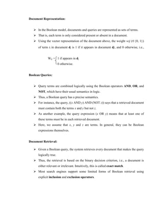
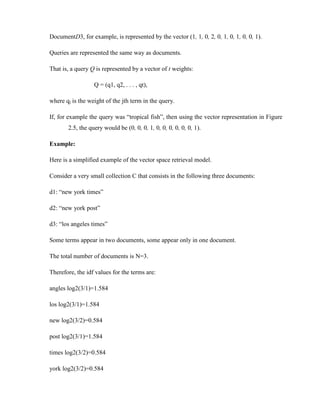
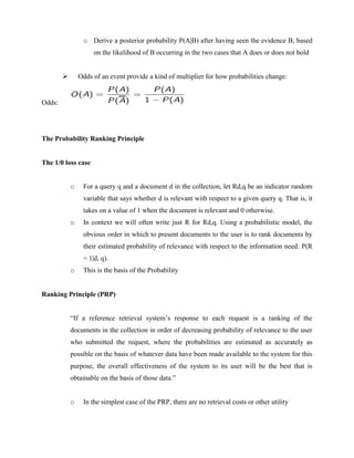
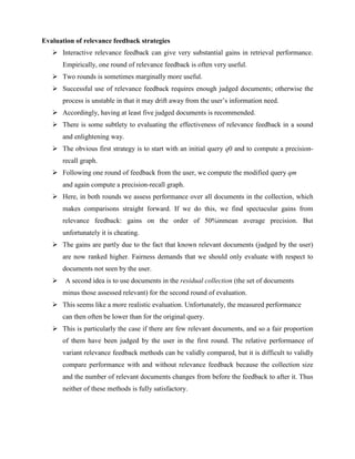
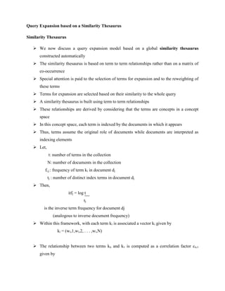
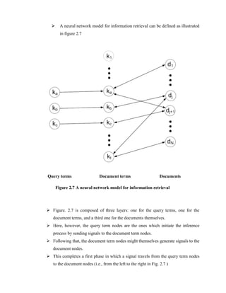
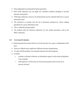
18. Probability Estimates in Practice
 Assuming that relevant documents are a very small percentage of the collection,
approximate statistics for non relevant documents by statistics from the whole
collection
 Hence, ut (the probability of term occurrence in non relevant documents for a
query) is dft/N and log[(1 − ut )/ut ] = log[(N − dft)/df t ] ≈ log N/df t
 The above approximation cannot easily be extended to relevant documents
Statistics of relevant documents (pt ) can be estimated in various ways:
1. Use the frequency of term occurrence in known relevant documents (if
known). This is the basis of probabilistic approaches to relevance
feedback weighting in a feedback loop
2. Set as constant. E.g., assume that pt is constant over all terms xt in the
query and that pt = 0.5
2.5 Latent Semantic Indexing Model
 The retrieval models discussed so far are based on keyword or term
matching, i.e., matching terms in the user query with those in the documents.
 If a user query uses different words from the words used in a document, the
document will not be retrieved although it may be relevant because the
document uses some synonyms of the words in the user query.
 This causes low recall. For example, “picture”, “image” and “photo” are
synonyms in the context of digital cameras. If the user query only has the
word “picture”, relevant documents that contain “image” or “photo” but not
“picture” will not be retrieved.
 Latent semantic indexing (LSI), aims to deal with this problem through the
identification of statistical associations of terms.
 It is assumed that there is some underlying latent semantic structure in the
data that is partially obscured by the randomness of word choice.

19.  It then uses a statistical technique, called singular value decomposition
(SVD), to estimate this latent structure, and to remove the “noise”.
 The results of this decomposition are descriptions of terms and documents
based on the latent semantic structure derived from SVD. This structure is
also called the hidden “concept” space, which associates syntactically
different but semantically similar terms and documents.
 These transformed terms and documents in the “concept” space are then used
in retrieval, not the original terms or documents.
 Let D be the text collection, the number of distinctive words in D be m and
the number of documents in D be n.
 LSI starts with an m×n term document matrix A. Each row of A represents a
term and each column represents a document.
 The matrix may be computed in various ways, e.g., using term frequency or
TF-IDF values.
 We use term frequency as an example in this section. Thus, each entry or cell
of the matrix A, denoted by Aij, is the number of times that term i occurs in
document j.
Singular Value Decomposition
o What SVD does is to factor matrix A (a m×n matrix) into the product of three
matrices, i.e.,
A= U∑VT
Where,
U is a m×r matrix and its columns, called right singular vectors, are
eigenvectors associated with the r non-zero eigen values of AAT.
Furthermore, the columns of U are unit orthogonal vectors,
i.e., UTU = I (identity matrix).

20. V is an n×r matrix and its columns, called right singular vectors, are
eigenvectors associated with the r non-zero eigenvalues of ATA. The
columns of V are also unit orthogonal vectors, i.e., VTV = I.
∑ is a r×r diagonal matrix,
∑=diag( 𝜎1, 𝜎 2, …, 𝜎 r), 𝜎i >0. 𝜎1, 𝜎 2, …..and 𝜎 r , called singular
values, are the non-negative square roots of the r (non-zero) eigen values
of AAT. They are arranged in decreasing order, i.e., 𝜎1≥ 𝜎 2≥ …≥𝜎 r≥0.
o We note that initially U is in fact an m�m matrix and V an n×n matrix and∑
an m×n diagonal matrix.
o ∑’s diagonal consists of nonnegative eigen values of AAT or ATA.
o However, due to zero eigen values, ∑ has zero-valued rows and columns.
Matrix multiplication tells us that those zero-valued rows and columns from
∑ can be dropped.
o Then, the last m×r columns in U and the last n-r columns in V can also be
dropped.
m is the number of row (terms) in A, representing the number of terms.
n is the number of columns in A, representing the number of documents.
r is the rank of A,
r≤ min(m, n).
The singular value decomposition of A always exists and is unique up to
1. allowable permutations of columns of U and V and elements of ∑ leaving it still
diagonal; that is, columns i and j of ∑ may be interchanged iff row i and j of ∑ are
interchanged, and columns i and j of U and V are interchanged.
2. sign (+/-) flip in U and V.

21. o An important feature of SVD is that we can delete some insignificant
dimensions in the transformed (or “concept”) space to optimally (in the least
square sense) approximate matrix A.
o The significance of the dimensions is indicated by the magnitudes of the
singular values in ∑, which are already sorted. In the context of information
retrieval, the insignificant dimensions may represent “noisy” in the data, and
should be removed.
o Let us use only the k largest singular values in ∑ and set the remaining small
ones to zero. The approximated matrix of A is denoted by Ak.
o We can also reduce the size of the matrices ∑, U and V by deleting the last r-k
rows and columns from ∑, the last r-k columns in U and the last r-k columns
in V.
We then obtain
Ak=Uk∑kVk
T
o Which means that we use the k-largest singular triplets to approximate the
original (and somewhat “noisy”) term-document matrix A.
o The new space is called the k-concept space.
o Figure 2.6 shows the original matrices and the reduced matrices
schematically.

22. Fig. 2.6. The schematic representation of A and Ak
o It is critical that the LSI method does not re-construct the original term
document matrix A perfectly.
o The truncated SVD captures most of the important underlying structures in
the association of terms and documents, yet at the same time removes the
noise or variability in word usage that plagues keyword matching retrieval
methods.
Query and Retrieval
o Given a user query q (represented by a column vector as those in A), it is first
converted into a document in the k-concept space, denoted by qk. This
transformation is necessary because SVD has transformed the original
documents into the k-concept space and stored them in Vk.
o The idea is that q is treated as a new document in the original space
represented as a column in A, and then mapped to qk as an additional
document (or column) in Vk
T
Documents
Term
vectors k
Document
k
k
∑k
Vk
T
vectors
∑ VT
Terms A/Ak = Uk U

23. q= ∑kqk
T
o Since the columns in U are unit orthogonal vectors, UkT
Uk = I.
Thus,
UkT
q=∑kqk
T
o As the inverse of a diagonal matrix is still a diagonal matrix, and each entry
on the diagonal is 1/ 𝜎 i(1≤i≤k), if it is multiplied on both sides of above
equation,we obtain, ∑k
-1
UkT
q= qk
T
o Finally, we get the following (notice that the transpose of a diagonal matrix is
itself), qk=qT
Uk∑k
-1
o For retrieval, we simply compare qk with each document (row) in Vk using a
similarity measure, e.g., the cosine similarity.
o Recall that each row of Vk (or each column of Vk
T
) corresponds to a
document (column) in A.
o This method has been used traditionally.
2.6 Neural Network Model
 The human brain is composed of billions of neurons. Each neuron can be
viewed as a small processing unit.
 A neuron is stimulated by input signals and emits output signals in reaction.
 A chain reaction of propagating signals is called a spread activation process.
As a result of spread activation, the brain might command the body to take
physical reactions
 A neural network is an oversimplified representation of the neuron
interconnections in the human brain: nodes are processing units edges are
synaptic connections the strength of a propagating signal is modeled by a
weight assigned to each edge the state of a node is defined by its activation
level depending on its activation level, a node might issue an output signal

24.  A neural network model for information retrieval can be defined as illustrated
in figure 2.7
Query terms Document terms Documents
Figure 2.7 A neural network model for information retrieval
 Figure. 2.7 is composed of three layers: one for the query terms, one for the
document terms, and a third one for the documents themselves.
 Here, however, the query term nodes are the ones which initiate the inference
process by sending signals to the document term nodes.
 Following that, the document term nodes might themselves generate signals to the
document nodes.
 This completes a first phase in which a signal travels from the query term nodes
to the document nodes (i.e., from the left to the right in Fig. 2.7 )

25.  The neural network however, does not stop after the first phase of signal
propagation. In fact, the document nodes in their turn might generate new signals
which are directed back to the document term nodes.
 Upon receiving the stimulus, the document term nodes might again fire new
signals directed to the document nodes, repeating the process.
 The signal become weaker at each iteration and the spread activation process
eventually halts.
 To improve the retrieval performance, the network continues with the spreading
activation process after the first round of propagation.
 This modifies the initial vector ranking in a process analogous to a user relevance
feedback cycle.
 To make the process more effective, a minimum activation threshold might be
defined such that document nodes below this threshold send no signals out.
 There is no conclusive evidence that a neural network provides superior
performance with general collections. In fact, the model has not been tested
extensively with large document collections.
2.7 Retrieval Evaluation
 To evaluate an IR system is to measure how well the system meets the information needs
of the users.
o This is troublesome, given that a same result set might be interpreted differently
by distinct users.
o To deal with this problem, some metrics have been defined that, on average, have
a correlation with the preferences of a group of users.
 Without proper retrieval evaluation, one cannot
o determine how well the IR system is performing
o compare the performance of the IR system with that of other systems, objectively
 Retrieval evaluation is a critical and integral component of any modern IR system
 Systematic evaluation of the IR system allows answering questions such as:
o a modification to the ranking function is proposed, should we go ahead and
launch it?

26. o a new probabilistic ranking function has just been devised, is it superior to the
vector model and BM25 rankings?
o for which types of queries, such as business, product, and geographic queries, a
given ranking modification works best?
 Lack of evaluation prevents answering these questions and precludes fine tuning of the
ranking function.
 Retrieval performance evaluation consists of associating a quantitative metric to the
results produced by an IR system.
 This metric should be directly associated with the relevance of the results to the user
Usually, its computation requires comparing the results produced by the system with
results suggested by humans for a same set of queries.
2.8 Retrieval Metrics
The Cranfield Paradigm
 Evaluation of IR systems is the result of early experimentation initiated in the 50’s by
Cyril Cleverdon.
 The insights derived from these experiments provide a foundation for the evaluation of
IR systems.
 Cleverdon obtained a grant from the National Science Foundation to compare distinct
indexing systems.
 These experiments provided interesting insights, that culminated in the modern metrics
of precision and recall
o Recall ratio: the fraction of relevant documents retrieved
o Precision ration: the fraction of documents retrieved that are relevant
 For instance, it became clear that, in practical situations, the majority of searches does not
require high recall.
 Instead, the vast majority of the users require just a few relevant answers.
 The next step was to devise a set of experiments that would allow evaluating each
indexing system in isolation more thoroughly.
 The result was a test reference collection composed of documents, queries, and relevance
judgements.

27.  It became known as the Cranfield-2 collection.
 The reference collection allows using the same set of documents and queries to evaluate
different ranking systems.
 The uniformity of this setup allows quick evaluation of new ranking functions
2.9 Precision and Recall
Consider,
I: an information request
R: the set of relevant documents for I
A: the answer set for I, generated by an IR system
R ∩ A: the intersection of the sets R and A
 The recall and precision measures are defined as follows
o Recall is the fraction of the relevant documents (the set R ) which has been
retrieved
i.e., Recall = |R ∩ A|
|R|
o Precision is the fraction of the retrieved documents (the set A) which is
relevant
i.e., Precision = |R ∩ A|
|A|
 The definition of precision and recall assumes that all docs in the set A have been
examined. However, the user is not usually presented with all docs in the answer set
A at once.
 Consider a reference collection and a set of test queries

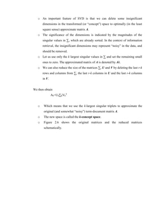
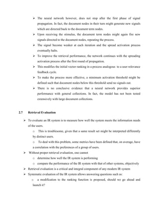
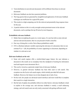
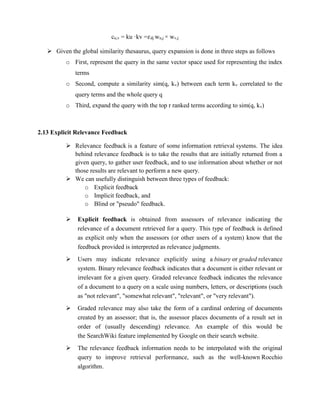
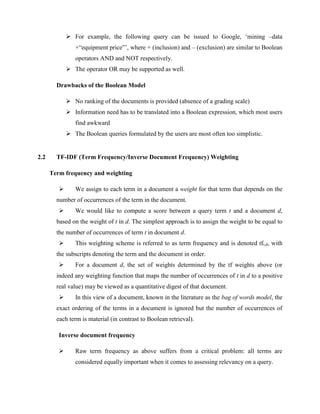
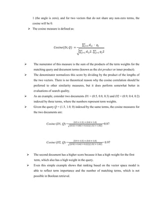
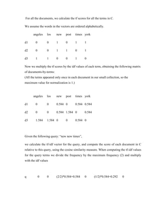
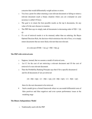
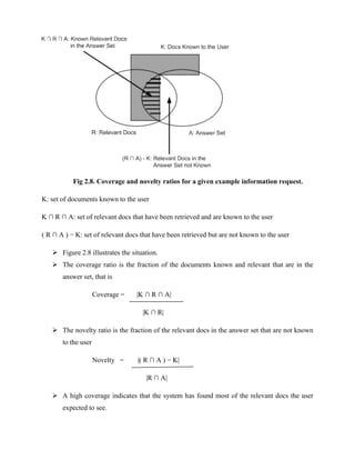
28. Let R q1 be the set of relevant docs for a query q1:
R q 1 = { d3, d5, d9, d25, d39, d44, d56, d71, d89, d123 }
o Consider a new IR algorithm that yields the following answer to q 1 (relevant
docs are marked with a bullet):
01. d123 • 06. d9 • 11. d38
02. d84 07. d511 12. d48
03. d56 • 08. d129 13. d250
04. d6 09. d187 14. d113
05. d8 10. d25 • 15. d3 •
 If we examine this ranking, we observe that The document d123, ranked as number
1, is relevant
 This document corresponds to 10% of all relevant documents.
 Thus, we say that we have a precision of 100% at 10% recall.
 The document d56, ranked as number 3, is the next relevant.
 At this point, two documents out of three are relevant, and two of the ten relevant
documents have been seen.
 Thus, we say that we have a precision of 66.6% at 20% recall.
2.10 Reference Collection
 Reference collections, which are based on the foundations established by the Cranfield
experiments, constitute the most used evaluation method in IR
 A reference collection is composed of:
o A set D of pre-selected documents
o A set I of information need descriptions used for testing
o A set of relevance judgements associated with each pair [im, dj], im € I and dj € D .
 The relevance judgement has a value of 0 if document dj is non-relevant to im , and 1
otherwise.

29.  These judgements are produced by human specialists.
 With small collections one can apply the Cranfield evaluation paradigm to provide
relevance assessments.
 With large collections, however, not all documents can be evaluated relatively to a given
information need.
 The alternative is consider only the top k documents produced by various ranking
algorithms for a given information need.
 This is called the pooling method.
 The method works for reference collections of a few million documents, such as the
TREC collections.
2.11 User-based Evaluation
 Recall and precision assume that the set of relevant docs for a query is independent of the
users.
 However, different users might have different relevance interpretations.
 To cope with this problem, user-oriented measures have been proposed.
 As before,
o consider a reference collection, an information request I, and a retrieval algorithm
to be evaluated
o With regard to I, let R be the set of relevant documents and A be the set of
answers retrieved.

30. Fig 2.8. Coverage and novelty ratios for a given example information request.
K: set of documents known to the user
K ∩ R ∩ A: set of relevant docs that have been retrieved and are known to the user
( R ∩ A ) − K: set of relevant docs that have been retrieved but are not known to the user
 Figure 2.8 illustrates the situation.
 The coverage ratio is the fraction of the documents known and relevant that are in the
answer set, that is
Coverage = |K ∩ R ∩ A|
|K ∩ R|
 The novelty ratio is the fraction of the relevant docs in the answer set that are not known
to the user
Novelty = |( R ∩ A ) − K|
|R ∩ A|
 A high coverage indicates that the system has found most of the relevant docs the user
expected to see.

31.  A high novelty indicates that the system is revealing many new relevant docs which
were unknown.
 Additionally, two other measures can be defined
o relative recall: ratio between the number of relevant docs found and the number of
relevant docs the user expected to find
o recall effort: ratio between the number of relevant docs the user expected to find
and the number of documents examined in an attempt to find the expected relevant
documents
2.12 Relevance feedback and query expansion
 In most collections, the same concept may be referred to using different
words. This issue, known as synonymy, has an impact on the recall of most
information retrieval systems.
 For example, you would want a search for aircraft to match plane (but only for
references to an airplane, not a wood work-ing plane), and for a search on
thermodynamics to match references to heat in appropriate discussions.
 Users often attempt to address this problem themselves by manually refining a
query, as was discussed in this Section.
 The methods for tackling this problem split into two major classes as shown in
Fig.2.9:
 Global methods
 Local methods.
 Global methods are techniques for expanding or reformulating query terms
independent of the query and results returned from it, so that changes in the
query wording will cause the new query to match other semantically similar
terms. Global methods include:
 Query expansion/reformulation with a thesaurus or Word Net
 Query expansion via automatic thesaurus generation
 Techniques like spelling correction
 Local methods adjust a query relative to the documents that initially appear to
match the query. Local methods include:

32.  Relevance feedback
 Pseudo relevance feedback, also known as Blind relevance
feedback
 (Global) indirect relevance feedback
Implicit Feedback
Fig. 2.9 (a) Local analysis (b) Global analysis

33. Relevance feedback and pseudo relevance feedback
Relevance feedback: user feedback on relevance of docs in initial set of results
Basic Procedure:
 User issues a (short, simple) query
 The system returns an initial set of retrieval results.
 The user marks some results as relevant or non-relevant
 The system computes a better query representation of the information need based on
feedback
 The system displays a revised set of retrieval results.
 Relevance feedback can go through one or more iterations of this sort.
 The process exploits the idea that it may be difficult to formulate a good query
when you don’t know the collection well, but it is easy to judge particular
documents, and so it makes sense to engage in iterative query refinement of this
sort.
 In such a scenario, relevance feedback can also be effective in tracking a user’s
evolving information need: seeing some documents may lead users to refine their
understanding of the information they are seeking.
 Image search provides a good example of relevance feedback.
 After the user enters an initial query for bike on the demonstration system at:
http://nayana.ece.ucsb.edu/imsearch/imsearch.html
the initial results (in this case, images) are returned.
 In Figure 2.10 (a), the user has selected some of them as relevant. These
will be used to refine the query, while other displayed results have no
effect on the reformulation.
 Figure 2.10 (b) then shows the new top-ranked results calculated after this
round of relevance feedback.

34. (a)
(b)
Figure 2.10 RF searching over images. (a) The user views the initial query results for
a query of bike, selects the first, third and fourth result in the top row and the fourth
result in the bottom row as relevant, and submits this feedback. (b) The users sees the
revised result set. Precision is greatly improved.

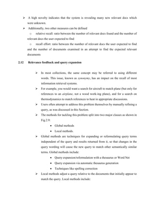
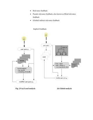
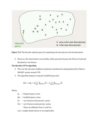
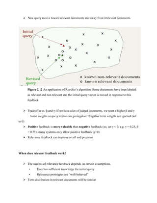
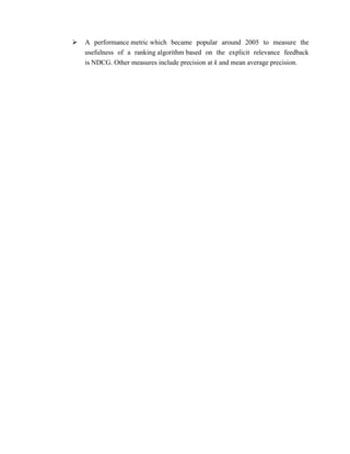
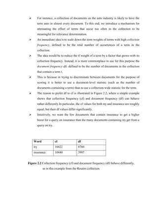
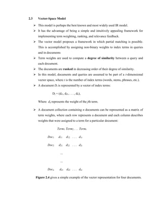
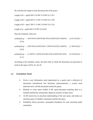
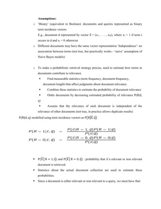
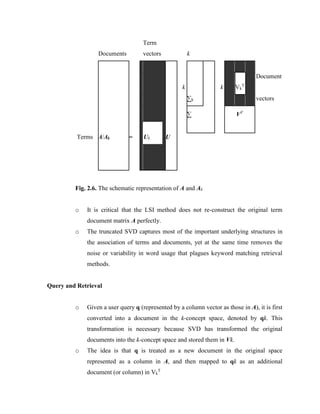
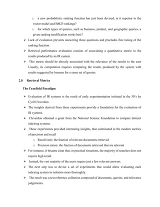
35. The Rocchio algorithm for relevance feedback
 It is the classic algorithm for implementing RF.
 The Rocchio algorithm uses the vector space model to pick a relevance feedback
query
 Rocchio seeks the query𝑞𝑜𝑝𝑡 that maximizes
𝑞𝑜𝑝𝑡 = 𝑎𝑟𝑔 𝑚𝑎𝑥[𝑠𝑖𝑚(𝑞, 𝐶𝑟) − 𝑠𝑖𝑚(𝑞, 𝐶𝑛𝑟)]
𝑞 = query vector, that maximizes similarity with relevant documents while
minimizing similarity with non relevant documents.
Cr = the set of relevant documents
Cnr = the set of non relevant documents
 Under cosine similarity, the optimal query vector 𝑞𝑜𝑝𝑡 for separating the
relevant and non relevant documents is:
𝑞𝑜𝑝𝑡 =
1
|𝐶𝑟|
∑ 𝑑𝑗
𝑑𝑗∈𝐶𝑟
−
1
|𝐶𝑛𝑟|
∑ 𝑑𝑗
𝑑𝑗∈𝐶𝑛𝑟
 That is, the optimal query is the vector difference between the centroids of
the relevant and non relevant documents as shown in Figure 2.11

36. Figure 2.11 The Rocchio optimal query for separating relevant and non relevant documents
 However, this observation is not terribly useful, precisely because the full set of relevant
documents is not known
The Rocchio (1971) algorithm.
 This was the relevance feedback mechanism introduced in and popularized by Salton’s
SMART system around 1970
 The algorithm proposes using the modified query 𝑞m:
𝑞𝑚 = 𝛼𝑞𝑜 + 𝛽
1
|𝐷𝑟|
∑ 𝑑𝑗 − 𝛾
1
|𝐷𝑛𝑟|
𝑑𝑗∈𝐷𝑟
∑ 𝑑𝑗
𝑑𝑗∈𝐷𝑛𝑟
Where,
𝑞𝑜 = Original query vector
𝑞𝑚 = modified query vector
Dr = set of known relevant doc vectors
Dnr = set of known irrelevant doc vectors
These are different from Cr and Cnr
α,β,γ: weights (hand-chosen or set empirically)

37.  New query moves toward relevant documents and away from irrelevant documents.
Figure 2.12 An application of Rocchio’s algorithm. Some documents have been labeled
as relevant and non relevant and the initial query vector is moved in response to this
feedback.
 Tradeoff α vs. β and γ: If we have a lot of judged documents, we want a higher β and γ
Some weights in query vector can go negative: Negative term weights are ignored (set
to 0)
 Positive feedback is more valuable than negative feedback (so, set γ < β; e.g. γ = 0.25, β
= 0.75) -many systems only allow positive feedback (γ=0)
 Relevance feedback can improve recall and precision
When does relevant feedback work?
 The success of relevance feedback depends on certain assumptions.
• User has sufficient knowledge for initial query
• Relevance prototypes are “well-behaved”
 Term distribution in relevant documents will be similar

38.  Term distribution in non-relevant documents will be different from those in relevant
documents
 Relevance feedback can also have practical problems.
 The long queries that are generated by straightforward application of relevance feedback
techniques are inefficient for a typical IR system.
 This results in a high computing cost for the retrieval and potentially long response times
for the user.
 A partial solution to this is to only reweight certain prominent terms in the relevant
documents, such as perhaps the top 20 terms by term frequency.
Probabilistic relevance feedback
 Rather than reweighting the query in a vector space, if a user has told us some relevant
and non relevant documents, then we can proceed to build a classifier.
 One way of doing this is with a Naive Bayes probabilistic model.
 If R is a Boolean indicator variable expressing the relevance of a document, then we can
estimate P (xt = 1|R), the probability of a term t appearing in a document, depending on
whether it is relevant or not.
Relevance feedback on the web
 Some web search engines offer a similar/related pages feature: the user indicates a
document in the results set as exemplary from the standpoint of meeting his information
need and requests more documents like it.
 This can be viewed as a particular simple form of relevance feedback.
 However, in general relevance feedback has been little used in web search. One
exception was the Excite web search engine, which initially provided full relevance
feedback. However, the feature was in time dropped, due to lack of use.
 On the web, few people use advanced search interfaces and most would like to complete
their search in a single interaction.
 But the lack of uptake also probably reflects two other factors: relevance feedback is hard
to explain to the average user, and relevance feedback is mainly a recall enhancing
strategy, and web search users are only rarely concerned with getting sufficient recall.

39. Evaluation of relevance feedback strategies
 Interactive relevance feedback can give very substantial gains in retrieval performance.
Empirically, one round of relevance feedback is often very useful.
 Two rounds is sometimes marginally more useful.
 Successful use of relevance feedback requires enough judged documents; otherwise the
process is unstable in that it may drift away from the user’s information need.
 Accordingly, having at least five judged documents is recommended.
 There is some subtlety to evaluating the effectiveness of relevance feedback in a sound
and enlightening way.
 The obvious first strategy is to start with an initial query q0 and to compute a precision-
recall graph.
 Following one round of feedback from the user, we compute the modified query qm
and again compute a precision-recall graph.
 Here, in both rounds we assess performance over all documents in the collection, which
makes comparisons straight forward. If we do this, we find spectacular gains from
relevance feedback: gains on the order of 50%inmean average precision. But
unfortunately it is cheating.
 The gains are partly due to the fact that known relevant documents (judged by the user)
are now ranked higher. Fairness demands that we should only evaluate with respect to
documents not seen by the user.
 A second idea is to use documents in the residual collection (the set of documents
minus those assessed relevant) for the second round of evaluation.
 This seems like a more realistic evaluation. Unfortunately, the measured performance
can then often be lower than for the original query.
 This is particularly the case if there are few relevant documents, and so a fair proportion
of them have been judged by the user in the first round. The relative performance of
variant relevance feedback methods can be validly compared, but it is difficult to validly
compare performance with and without relevance feedback because the collection size
and the number of relevant documents changes from before the feedback to after it. Thus
neither of these methods is fully satisfactory.

40.  A third method is to have two collections, one which is used for the initial query and
relevance judgments, and the second that is then used for comparative evaluation. The
performance of both q0 and qm can be validly compared on the second collection.
 Perhaps the best evaluation of the utility of relevance feedback is to do user studies of its
effectiveness, in particular by doing a time-based comparison: how fast does a user find
relevant documents with relevance feedback vs.another strategy (such as query
reformulation), or alternatively, how many relevant documents does a user find in a
certain amount of time.
Pseudo relevance feedback
 It is also known as blind relevance feedback, provides a method for automatic local
analysis.
 It automates the manual part of relevance feedback, so that the user gets improved
retrieval performance without an extended interaction.
 The method is to do normal retrieval to find an initial set of most relevant documents, to
then assume that the top k ranked documents are relevant, and finally to do relevance
feedback as before under this assumption.
Indirect relevance feedback
 We can also use indirect sources of evidence rather than explicit feedback on relevance
as the basis for relevance feedback.
 This is often called implicit (relevance) feedback.
 Implicit feedback is less reliable than explicit feedback, but is more useful than pseudo
relevance feedback, which contains no evidence of user judgments.
Moreover, while users are often reluctant to provide explicit feedback, it is easy to collect
implicit feedback in large quantities for a high volume system, such as a web search engine.

41. Query Expansion based on a Similarity Thesaurus
Similarity Thesaurus
 We now discuss a query expansion model based on a global similarity thesaurus
constructed automatically
 The similarity thesaurus is based on term to term relationships rather than on a matrix of
co-occurrence
 Special attention is paid to the selection of terms for expansion and to the reweighting of
these terms
 Terms for expansion are selected based on their similarity to the whole query
 A similarity thesaurus is built using term to term relationships
 These relationships are derived by considering that the terms are concepts in a concept
space
 In this concept space, each term is indexed by the documents in which it appears
 Thus, terms assume the original role of documents while documents are interpreted as
indexing elements
 Let,
t: number of terms in the collection
N: number of documents in the collection
fi,j : frequency of term ki in document dj
tj : number of distinct index terms in document dj
 Then,
itfj = log t
tj
is the inverse term frequency for document dj
(analogous to inverse document frequency)
 Within this framework, with each term ki is associated a vector ki given by
ki = (wi,1,wi,2, . . . ,wi,N)
 The relationship between two terms ku and kv is computed as a correlation factor cu,v
given by

42. cu,v = ku ·kv =𝜀dj wu,j × wv,j
 Given the global similarity thesaurus, query expansion is done in three steps as follows
o First, represent the query in the same vector space used for representing the index
terms
o Second, compute a similarity sim(q, kv) between each term kv correlated to the
query terms and the whole query q
o Third, expand the query with the top r ranked terms according to sim(q, kv)
2.13 Explicit Relevance Feedback
 Relevance feedback is a feature of some information retrieval systems. The idea
behind relevance feedback is to take the results that are initially returned from a
given query, to gather user feedback, and to use information about whether or not
those results are relevant to perform a new query.
 We can usefully distinguish between three types of feedback:
o Explicit feedback
o Implicit feedback, and
o Blind or "pseudo" feedback.
 Explicit feedback is obtained from assessors of relevance indicating the
relevance of a document retrieved for a query. This type of feedback is defined
as explicit only when the assessors (or other users of a system) know that the
feedback provided is interpreted as relevance judgments.
 Users may indicate relevance explicitly using a binary or graded relevance
system. Binary relevance feedback indicates that a document is either relevant or
irrelevant for a given query. Graded relevance feedback indicates the relevance
of a document to a query on a scale using numbers, letters, or descriptions (such
as "not relevant", "somewhat relevant", "relevant", or "very relevant").
 Graded relevance may also take the form of a cardinal ordering of documents
created by an assessor; that is, the assessor places documents of a result set in
order of (usually descending) relevance. An example of this would be
the SearchWiki feature implemented by Google on their search website.
 The relevance feedback information needs to be interpolated with the original
query to improve retrieval performance, such as the well-known Rocchio
algorithm.

43.  A performance metric which became popular around 2005 to measure the
usefulness of a ranking algorithm based on the explicit relevance feedback
is NDCG. Other measures include precision at k and mean average precision.