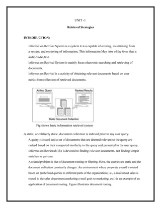
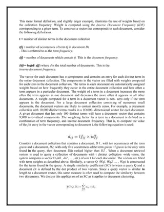
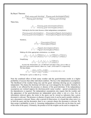
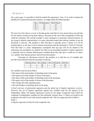
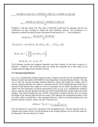
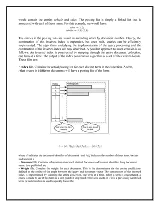
This document provides lecture notes on information retrieval systems. It covers key concepts like precision and recall, different retrieval strategies including vector space model and probabilistic models, and retrieval utilities. The vector space model represents documents and queries as vectors in a shared space and calculates similarity using cosine similarity. Probabilistic models assign probabilities to terms and documents and estimate relevance probabilities. The notes discuss term weighting schemes, inverted indexes to improve efficiency, and integrating structured data with text retrieval. The overall objective is for students to learn fundamental models and techniques for information storage and retrieval.


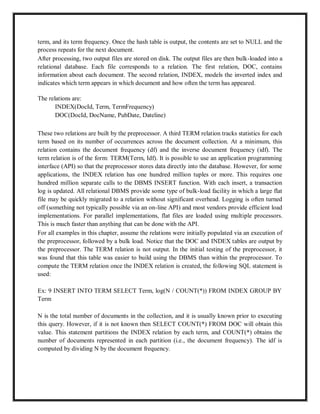
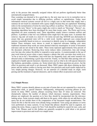
![to know how many documents are relevant to term t for other queries. The following equation
estimates the value of r i prior to doing a retrieval:
ri = a + blog f
where f is the frequency of the term across the entire document collection.
After obtaining a few sample points, values for a and b can be obtained by a least squares curve
fitting process. Once this is done, the value for ri can be estimated given a value of f, and using
the value of ri, an estimate for an initial weight (IW) is obtained. The initial weights are then
combined to compute a similarity coefficient. In the paper [Wu and Salton, 1981] it was
concluded (using very small collections) that idf was far less computationally expensive, and that
the IW resulted in slightly worse precision and recall.
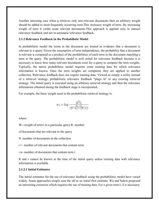
2.1.2.2 Computing New Query Weights
For,query Q,Document D and t terms in D,Di is binary.If the term is present then place 1
otherwise place 0.
Where k is constant.
After substituting we get
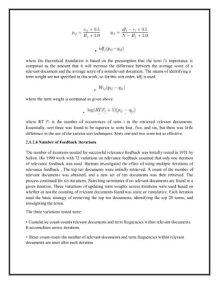
Using relevance feedback, a query is initially submitted and some relevant documents might be
found in the initial answer set. The top documents are now examined by the user and values for r
i and R can be more accurately estimated (the values for ni and N are known prior to any
retrieval). Once this is done, new weights are computed and the query is executed again. Wu and
Salton tested four variations of composing the new query:
1. Generate the new query using weights computed after the first retrieval.
2. Generate the new query, but combine the old weights with the new. Wu suggested that the
weights could be combined as:](https://image.slidesharecdn.com/irs-lecture-notes-240221152232-7e66d3d2/85/IRS-Lecture-Notes-irsirs-IRS-Lecture-Notes-irsirs-IRS-Lecture-Notes-irsirs-IRS-Lecture-Notes-irsirs-IRS-Lecture-Notes-irsirs-26-320.jpg)
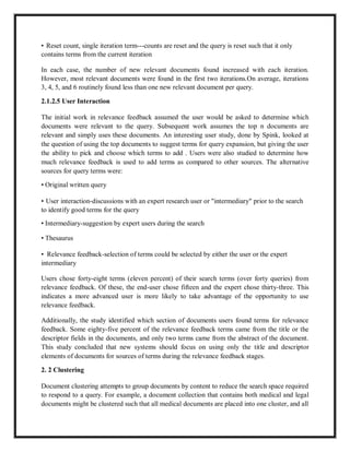
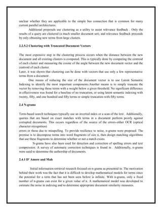
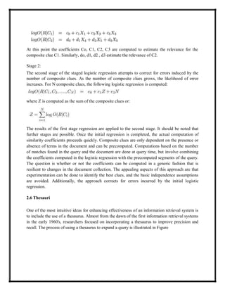
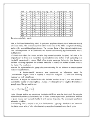
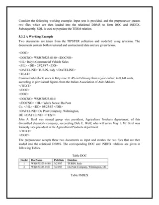
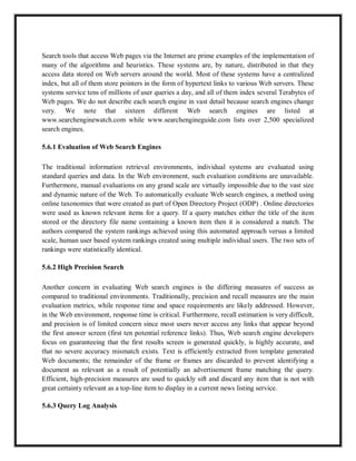
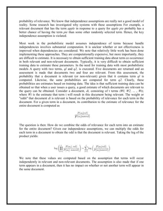
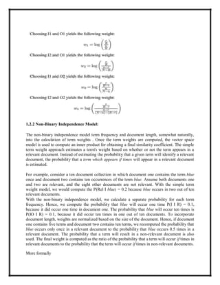
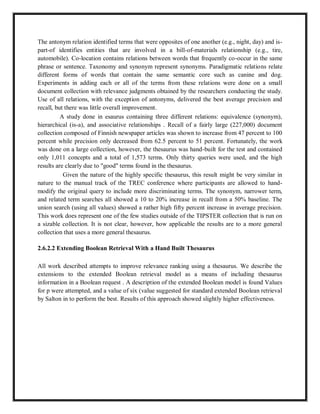
![thesaurus assisted their recall. No testing of generic precision and recall for automatic retrieval
was measured.
2.6.1.2 Term Context
Instead of relying on term co-occurrence, some work uses the context (surrounding terms) of
each term to construct the vectors that represent each term ]. The problem with the vectors given
above is that they do not differentiate the senses of the words. A thesaurus relates words to
different senses. In the example given below, "bark" has two entirely different senses. A typical
thesaurus lists "bark" as:
bark-surface of tree (noun)
bark-dog sound (verb
Ideally an automatically generated thesaurus would have separate lists of synonyms.
The term-term matrix does not specifically identify synonyms, and Gauch and Wang do not
attempt this either. Instead, the relative position of nearby terms is included in the vector used to
represent a term .
The key to similarity is not that two terms happen to occur in the same document; it is
that the two terms appear in the same context-that is they have very similar neighboring terms.
Bark, in the sense of a sound emanating from a dog, appears in different contexts than bark, in
the sense of a tree surface. Consider the following three sentences:
s 1: "The dog yelped at the cat."
s2 : "The dog barked at the cat."
s3 : "The bark fell from the tree to the ground."
In sentences s1 and s2, yelped is a synonym for barked, and the two terms occur in
exactly the same context. It is unlikely that another sense of bark would appear in the same
context. "Bark" as a suiface of tree more commonly would have articles at one position to the left
instead of two positions to the left, etc.
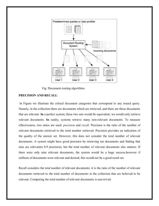
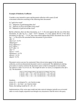
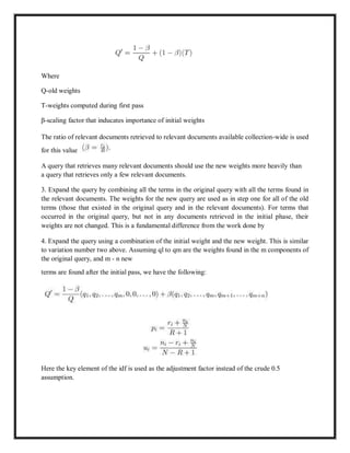
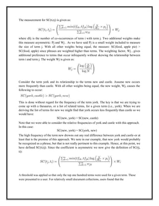
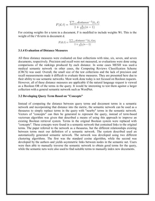
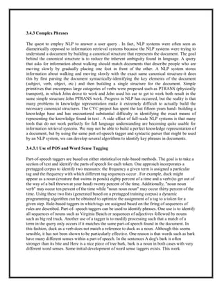
To capture the term's context, it is necessary to identify a set of context terms. The
presence or absence of these terms around a given target term will determine the content of the
vector for the target term. The authors assume the highest frequency terms are the best context
terms, so the 200 most frequent terms (including stop terms) are used as context terms. A
window of size seven was used. This window includes the three terms to the left of the target
term and the three terms to the right of the target term. The new vector that represents target term
i will be of the general form:](https://image.slidesharecdn.com/irs-lecture-notes-240221152232-7e66d3d2/85/IRS-Lecture-Notes-irsirs-IRS-Lecture-Notes-irsirs-IRS-Lecture-Notes-irsirs-IRS-Lecture-Notes-irsirs-IRS-Lecture-Notes-irsirs-48-320.jpg)
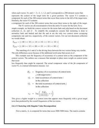
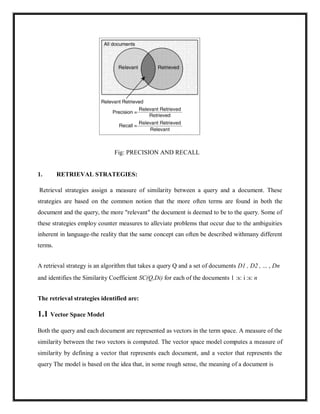
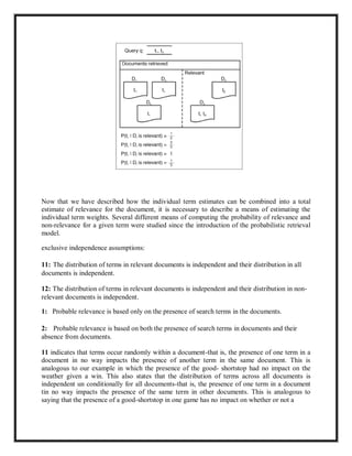
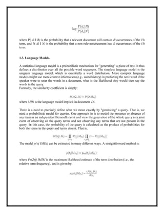
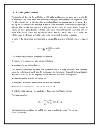
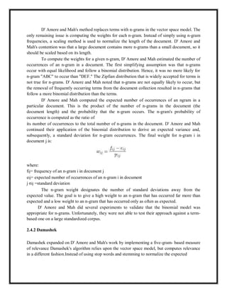
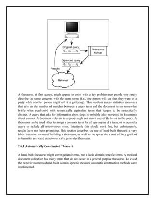
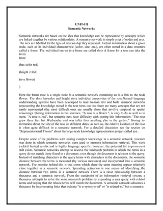
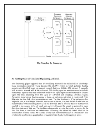
![the number of times these terms co-occur with a term window of size k (k is 40 in this work).
Subsequently, these terms are clustered into 200 A-classes (group average agglomerative
clustering is used). For example, one A-class, gAl, might have terms (tl, t2, t3) and another, gA2,
would
have (t4,t5).
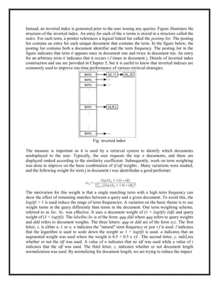
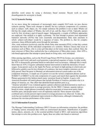
Subsequently, a new matrix, B, is generated for the 20,000 most frequent terms based on
their co-occurrence between clusters found in the matrix. For example, if term tj co-occurs with
term tl ten times, term t2 five times, and term t4 six times, B[I, j] = 15 and B[2, j] = 6. Note the
use of clusters has reduced the size of the B matrix and provides substantially more training
information. The rows of B correspond to classes in A, and the columns correspond to terms.
The B matrix is of size 200 x 20,000. The 20,000 columns are then clustered into 200 B-classes
using the buckshot clustering algorithm] indicates the number oftimes termj co-occurs with the
B-classes. Once this is done, the C matrix is decomposed and singular values are computed to
represent the matrix. This is similar to the technique used for latent semantic indexing . The SVD
is more tractable at this point since only 200 columns exist. A document is represented by a
vector that is the sum of the context vectors (vectors that correspond to each column in the
SVD). The context vector is used to match a query.
Another technique that uses the context vector matrix, is to cluster the query based on its
context vectors. This is referred to as word factorization. The queries were partitioned into three
separate clusters. A query is then run for each of the word factors and a given document is given
the highest rank of the three. This requires a document to be ranked high by all three factors to
receive an overall high rank. The premise is that queries are generally about two or three
concepts and that a relevant document has information relevant to all of the concepts.
Overall, this approach seems very promising. It was run on a reasonably good-sized
collection (the Category B portion of TIPSTER using term factorization, average precision
improved from 0.27 to 0.32-an 18.5% overall improvement).
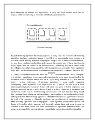
2.6.1.4 Using only Document Clustering to Generate a Thesaurus
Another approach to automatically build a thesaurus is, a document clustering algorithm is
implemented to partition the document collection into related clusters. A document-document
similarity coefficient is used. Complete link clustering is used here, but other clustering
algorithms could be used (for more details on clustering algorithms . The terms found in each
cluster are then obtained. Since they occur in different documents within the cluster, different
operators are used to obtain the set of terms that correspond to a given cluster. Consider
documents with the following terms:](https://image.slidesharecdn.com/irs-lecture-notes-240221152232-7e66d3d2/85/IRS-Lecture-Notes-irsirs-IRS-Lecture-Notes-irsirs-IRS-Lecture-Notes-irsirs-IRS-Lecture-Notes-irsirs-IRS-Lecture-Notes-irsirs-50-320.jpg)
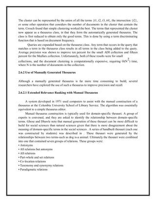

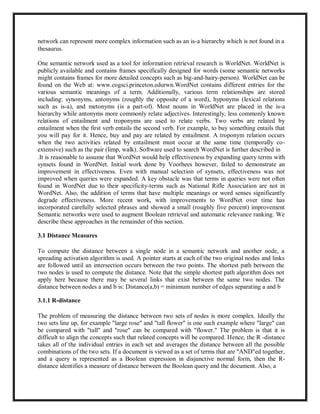
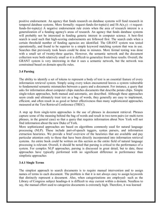
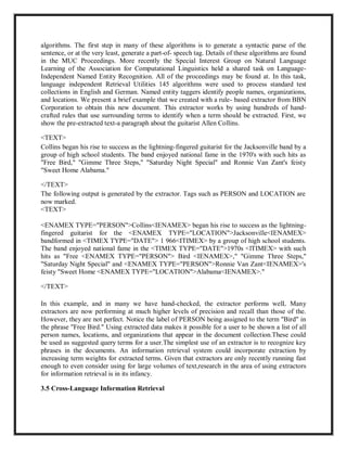

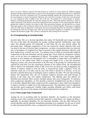
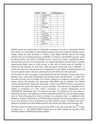
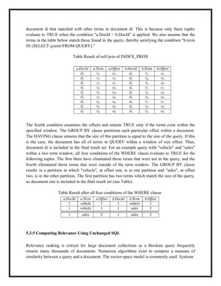
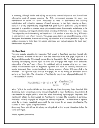
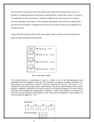
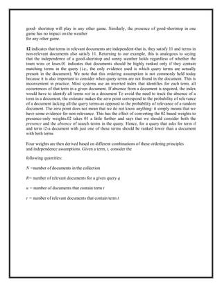
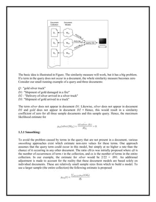
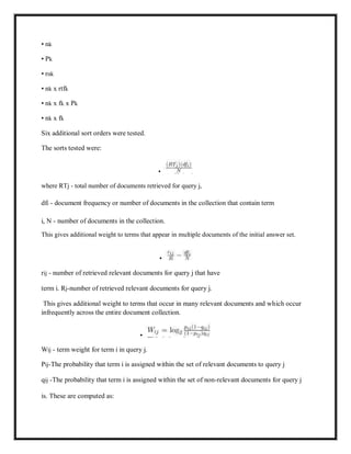
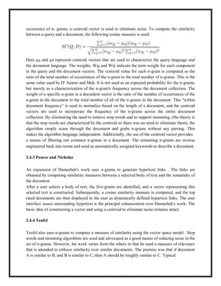
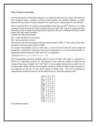
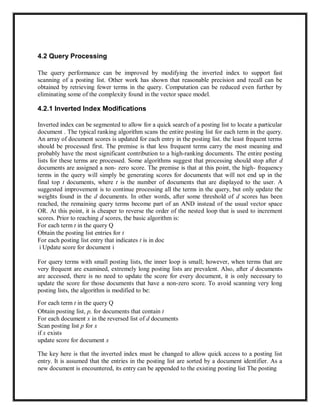
![bytes. The values and their corresponding compressed bit strings are shown in Table above. In
this example, uncompressed data requires 160 bits, while BA compression requires only 48 bits.
4.1.3 Variable Length Index Compression
The differences in the posting list. They capitalize on the fact that for most long posting lists, the
difference between two entries is relatively small.
They first mention that patterns can be seen in these differences and that Huffman encoding
provides the best compression. In this method, the frequency distribution of all of the offsets is
obtained through an initial pass over the text, a compression scheme is developed based on the
frequency distribution, and a second pass uses the new compression scheme. For example, if it
was found that an offset of one has the highest frequency throughout the entire index, the scheme
would use a single bit to represent the offset of one. This code represents an integer x with [
2llog2x] + 1 bits. The first [log2 x] bits are the unary representation of [log2x]. (Unary
representation is a base one representation of integers using only the digit one. The number 510
is represented as 111111.) After the leading unary representation, the next bit is a single stop bit
of zero. At this point, the highest power of two that does not exceed x has been represented. The
next [log2x] bits represent the remainder of x - 2 ^l[og2 x] in binary. As an example, consider the
compression of the decimal 14. First, [log2 x] =3 is represented in unary as 111. Next, the stop
bit is used. Subsequently, the remainder of x – 2^[lo g2 X ] = 14 - 8 = 6 is stored in binary using
[log2 14] = 3 bits as 110. Hence, the compressed code for 1410 is 1110110. Decompression
requires only one pass, because it is known that for a number with n bits prior to the stop bit,
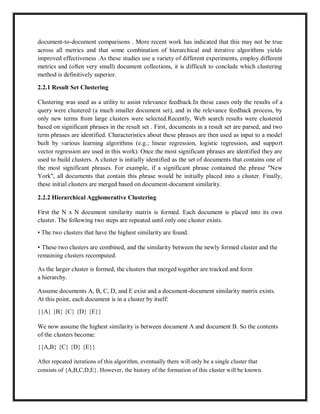
there will be n bits after the stop bit. The first eight integers using the Elias, encoding .](https://image.slidesharecdn.com/irs-lecture-notes-240221152232-7e66d3d2/85/IRS-Lecture-Notes-irsirs-IRS-Lecture-Notes-irsirs-IRS-Lecture-Notes-irsirs-IRS-Lecture-Notes-irsirs-IRS-Lecture-Notes-irsirs-73-320.jpg)
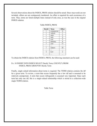
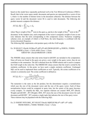
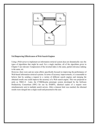
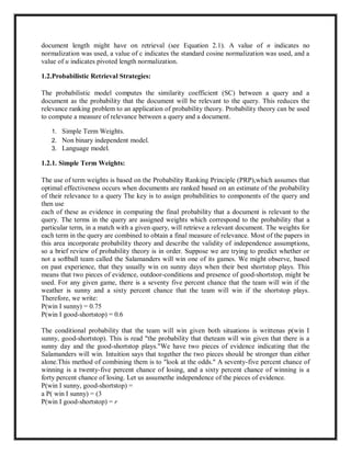
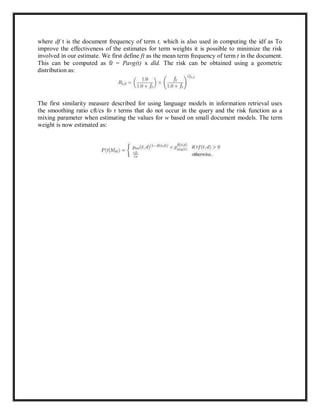
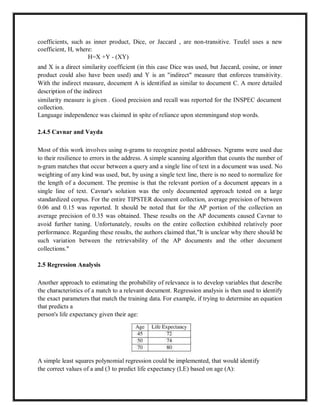
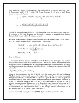
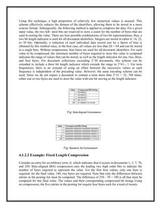
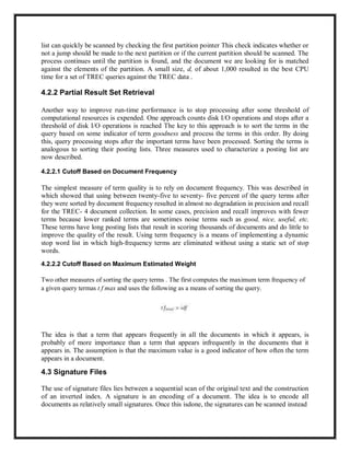
![4.1.3.1 Example: Variable Length Compression
For our same example, the differences of 1, 2, 4, 63, and 180 are given in Table. This requires
only 35 bits, thirteen less than the simple BA compression. Also, our example contained an even
distribution of relatively large offsets to small ones. The real gain can be seen in that very small
offsets require only a 1 or a O. Moffat and Zobel use the, code to compress the term frequency in
a posting list, but use a more complex coding scheme for the posting list entries.
4.1.4 Varying Compression Based on Posting List Size
The gamma scheme can be generalized as a coding paradigm based on the vector V with positive
integers i where 2: Vi 2: N. To code integer x 2: 1 relative to V, find k such that
In other words, find the first component of V such that the sum of all preceding components is
greater than or equal to the value, x, to be encoded. For our example of 7, using a vector V of
<1,2,4, 8, 16,32> we find the first three components that are needed (1, 2, 4) to equal or
exceed 7, so k is equal to three. Now k can be encoded in some representation (unary is
typically used) followed by the difference:
Using this sum we have: d = 7 - (1 + 2) - 1 = 3 which is now coded in[log2] Vk =[log2 4] = 2
binary bits. With this generalization, the, scheme
Table: Variable Compression based on Posting List Size
can be seen as using the vector V composed of powers of 2 < 1, 2, 4, 8, ... , > and coding k in
binary. Clearly, V can be changed to give different compression characteristics. Low values in v
optimize compression for low numbers, while higher values in v provide more resilience for high
numbers. A clever solution given by was to vary V for each posting list such that V = < b, 2b,
4b, 8b, 16b, 32b, 64b, ... , > where b is the median offset given in the posting list.](https://image.slidesharecdn.com/irs-lecture-notes-240221152232-7e66d3d2/85/IRS-Lecture-Notes-irsirs-IRS-Lecture-Notes-irsirs-IRS-Lecture-Notes-irsirs-IRS-Lecture-Notes-irsirs-IRS-Lecture-Notes-irsirs-74-320.jpg)
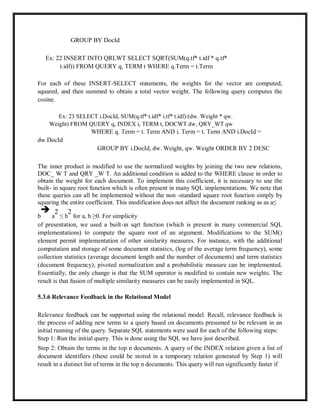
![continues to move forward with each comparison to facilitate a physically contiguous scan of a
disk. The KMP algorithm builds a finite state automata for many patterns so it is directly
applicable. An algorithm by Uratani and Takeda combines the FSA approach by Aho and
Corasick with the Boyer-Moore idea of avoiding much of the search space. Essentially, the FSA
is built by using some of the search space reductions given by Boyer-Moore. The FSA scans text
from right to left, as done in Boyer -Moore. Note this is done for a query that contains multiple
terms]. In a direct comparison with repeated use of the Boyer-Moore algorithm, the Uratani and
Takeda algorithm is shown to execute ten times fewer probes for a query of 100 patterns.
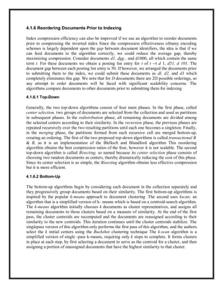
4.4 Duplicate Document Detection
A method to improve both efficiency and effectiveness of an information retrieval system is to
remove duplicates or near duplicates. Duplicates can be removed either at the time documents
are added to an inverted index or upon retrieving the results of a query. The difficulty is that we
do not simply wish to remove exact duplicates, we may well be interested in removing near
duplicates as well. However, we do not wish our threshold for nearness to be so broad that
documents are deemed duplicate when, in fact, they are sufficiently different that the user would
have preferred to see each of them as individual documents. For Web search, the duplicate
document problem is particularly acute. A search for the term apache might yield numerous
copies of Web pages about, the Web server product and numerous duplicates about the Indian
tribe. The user should only be shown two hyperlinks, but instead is shown thousands.
Additionally, these redundant pages can affect term and document weighting schemes.
Additionally, they can increase indexing time and reduce search efficiency.
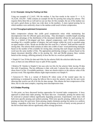
4.4.1 Finding Exact Duplicates
for each document. Each document is then examined for duplication by looking up the value
(hash) in either an in-memory hash or persistent lookup system. Several common hash functions
used are, These functions are used because they have three desirable properties, namely: they can
be calculated on arbitrary document lengths, they are easy to compute, and they have very low
probabilities of collisions. While this approach is both fast and easy to implement, the problem is
that it will find only exact duplicates. The slightest change (e.g.; one extra white space) results in
two similar documents being deemed unique. For example, a Web page that displays the number
of visitors along with the content of the page will continually produce different signatures even
though the document is the same. The only difference is the counter, and it will be enough to
generate a different hash value for each document.
4.4.2 Finding Similar Duplicates
While it is not possible to define precisely at which point a document is no longer a duplicate of
another, researchers have examined several metrics for determining the similarity of a document to
another. The first is resemblance . This work suggests that if a document contains roughly the same
semantic content, it is a duplicate whether or not it is a precise syntactic match](https://image.slidesharecdn.com/irs-lecture-notes-240221152232-7e66d3d2/85/IRS-Lecture-Notes-irsirs-IRS-Lecture-Notes-irsirs-IRS-Lecture-Notes-irsirs-IRS-Lecture-Notes-irsirs-IRS-Lecture-Notes-irsirs-81-320.jpg)


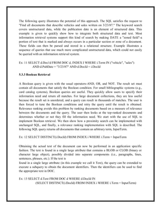
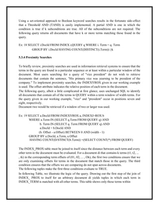
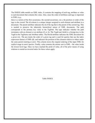
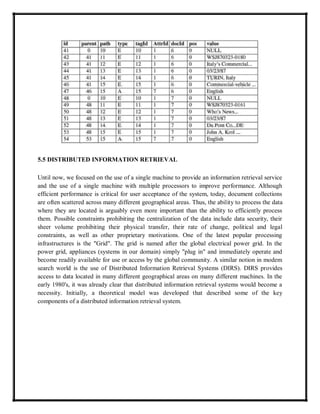
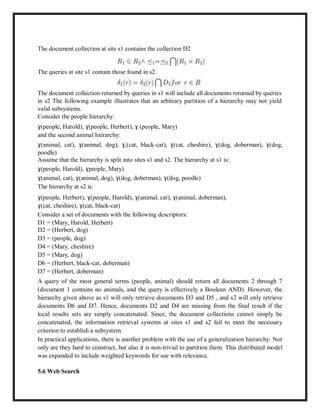
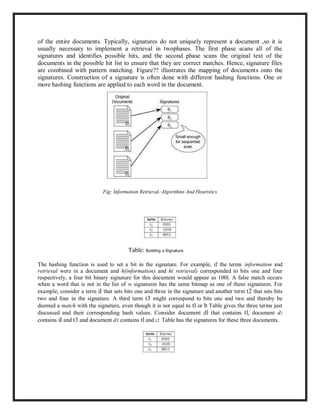
![Ex: 6 SELECT DISTINCT(i.DocId) FROM INDEX i, QUERY q, STOP ]ERM
s WHERE i.term = q.term AND i.term i= s.term
Finally, to implement a logical AND of the terms InputTerml, InputTerm2 and InputTerm3,
Ex: 7 SELECT DocId FROM INDEX WHERE term = InputTermI INTERSECT
SELECT DocId FROM INDEX WHERE term = InputTerm2 INTERSECT
SELECT DocId FROM INDEX WHERE term = InputTerm3
The query consists of three components. Each component results in a set of documents that
contain a single term in the query. The INTERSECT keyword is used to find the intersection of
the three sets. After processing, an AND is implemented.
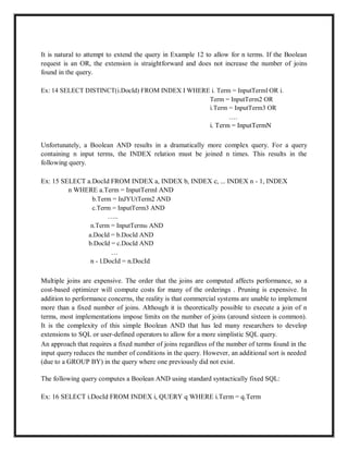
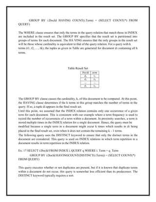
The key extension for relevance ranking was a corr() function-a built-in function to determine
the similarity of a document to a query.
The SEQUEL (a precursor to SQL) example that was given was:
Ex: 8 SELECT DocId FROM INDEX i, QUERY q WHERE i.term =
q.term GROUP BY DocId HAVING CORRO > 60
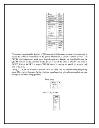
Other extensions, such as the ability to obtain the first n tuples in the answer set, were given. We
now describe the unchanged relational model to implement information retrieval functionality
with standard SQL. First, a discussion of preprocessing text into files for loading into a relational
DBMS is required.
5.3.1 Preprocessing
Input text is originally stored in source files either at remote sites or locally on CD-ROM. For
purposes of this discussion, it is assumed that the data files are in ASCII or can be easily
converted to ASCII with SGML markers. SGML markers are a standard means by which
different portions of the document are marked. The markers in the working example are found in
the TIPSTER collection which was in previous years as the standard dataset for TREC. These
markers begin with a < and end with a > (e.g., <TAG).A preprocessor that reads the input file
and outputs separate flat files is used. Each term is read and checked against a list of SGML
markers. The main algorithm for the preprocessor simply parses terms and then applies a hash
function to hash them into a small hash table. If the term has not occurred for this document, a
new entry is added to the hash table. Collisions are handled by a single linked list associated with
the hash table. If the term already exists, its term frequency is updated. When an end-of-
document marker is encountered, the hash table is scanned. For each entry in the hash table a
record is generated. The record contains the document identifier for the current document, the](https://image.slidesharecdn.com/irs-lecture-notes-240221152232-7e66d3d2/85/IRS-Lecture-Notes-irsirs-IRS-Lecture-Notes-irsirs-IRS-Lecture-Notes-irsirs-IRS-Lecture-Notes-irsirs-IRS-Lecture-Notes-irsirs-91-320.jpg)