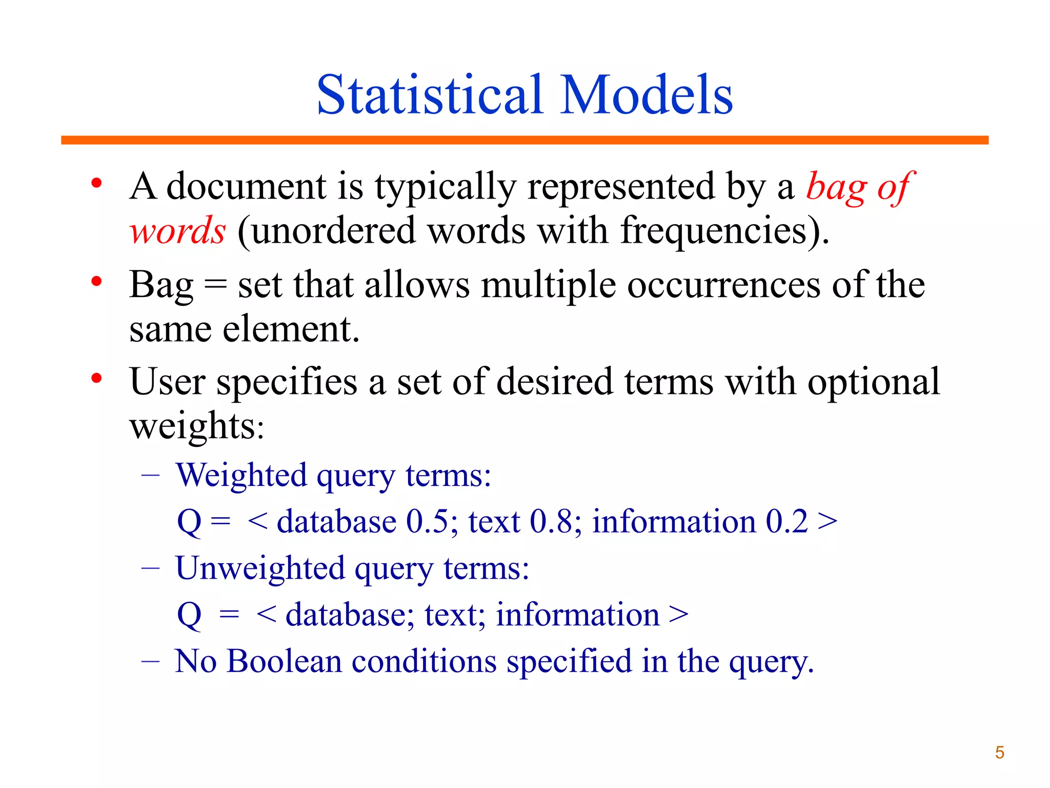
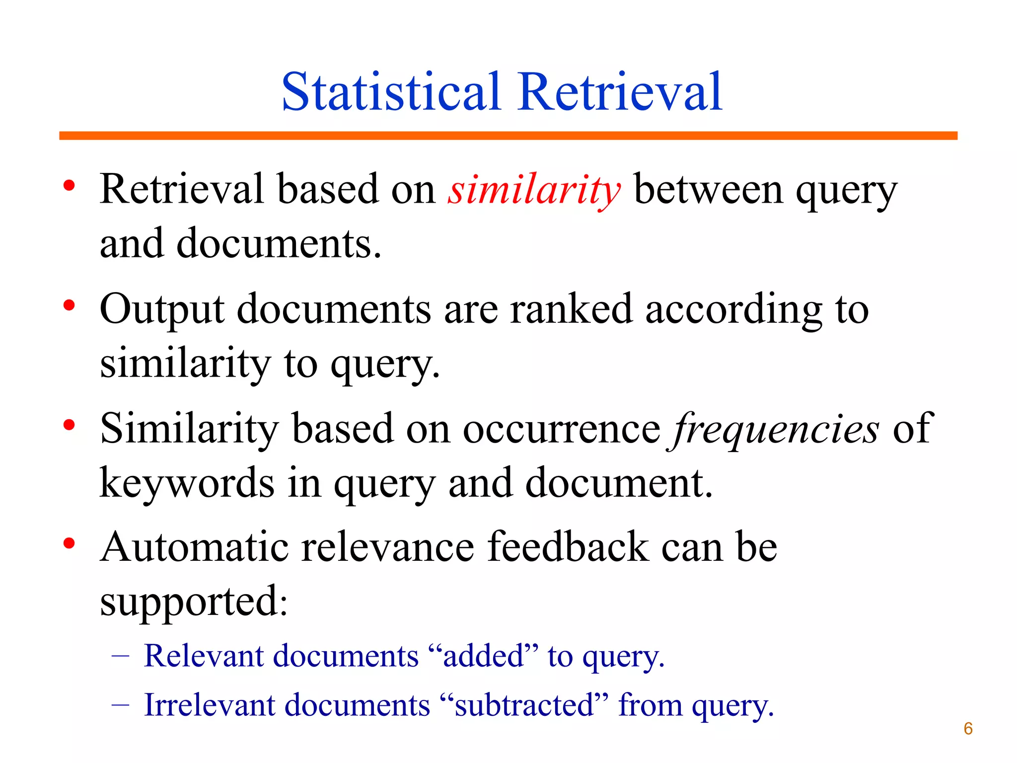
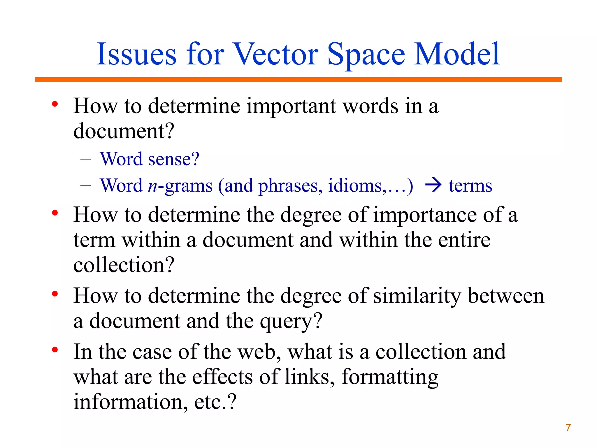
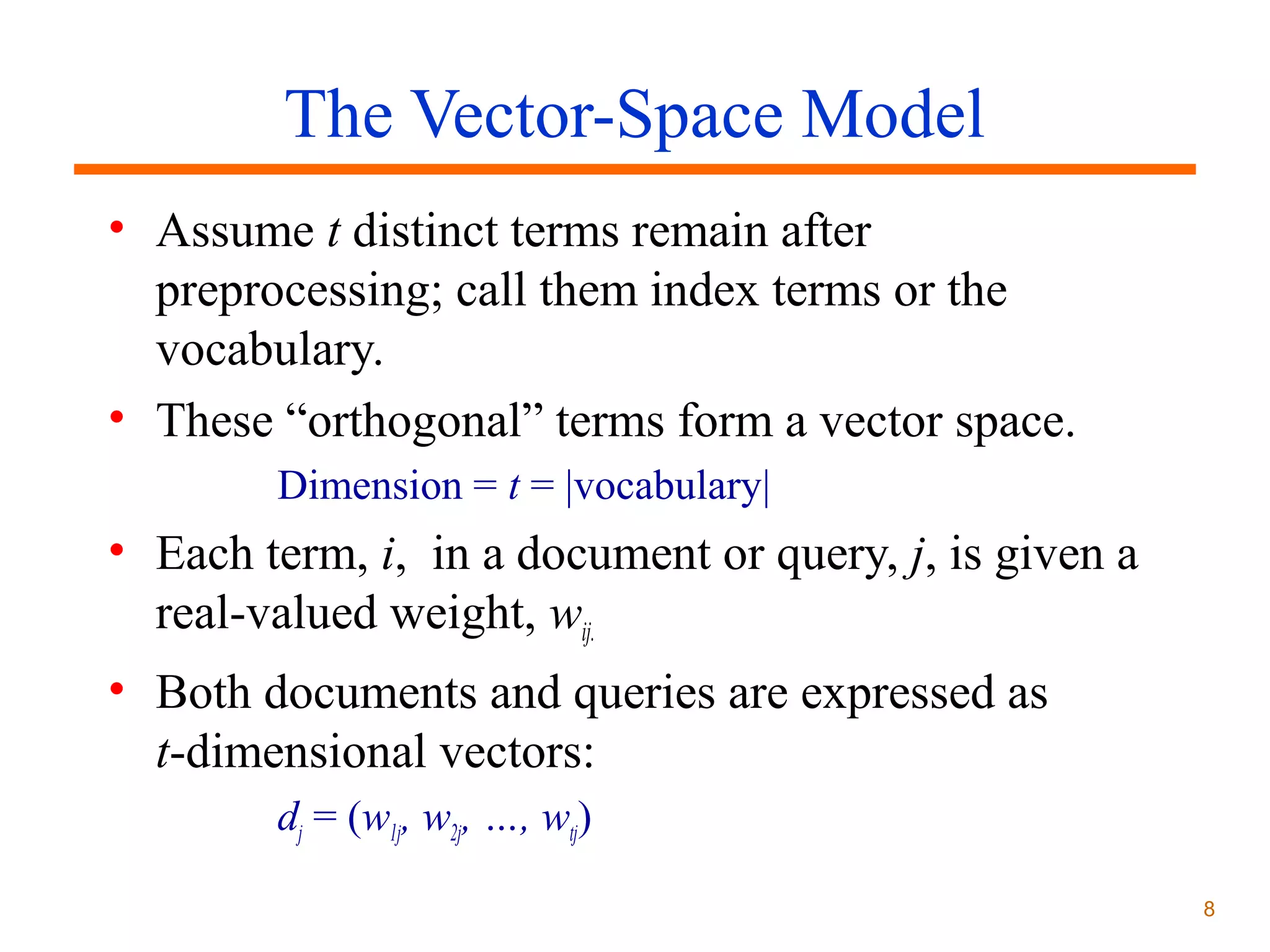
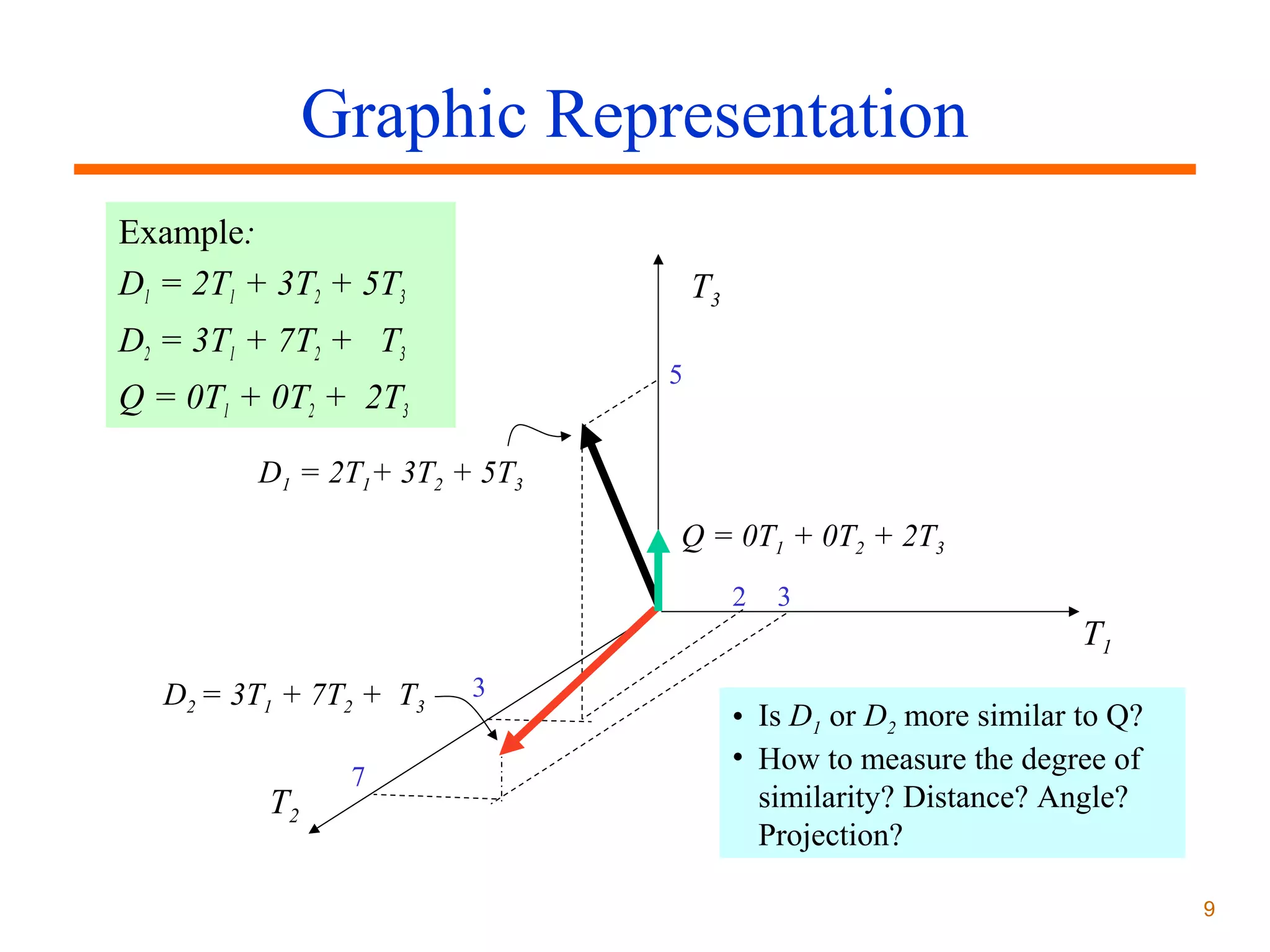
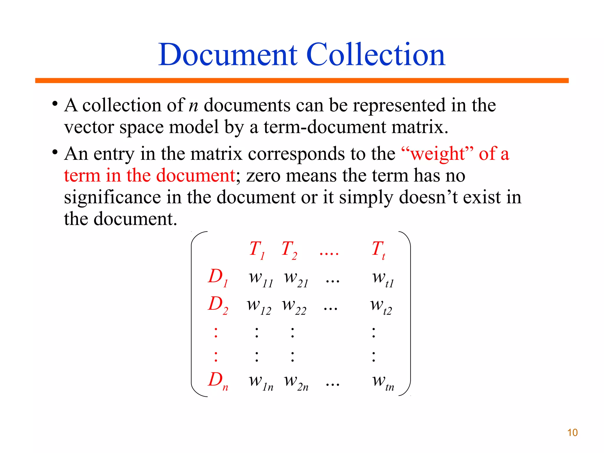
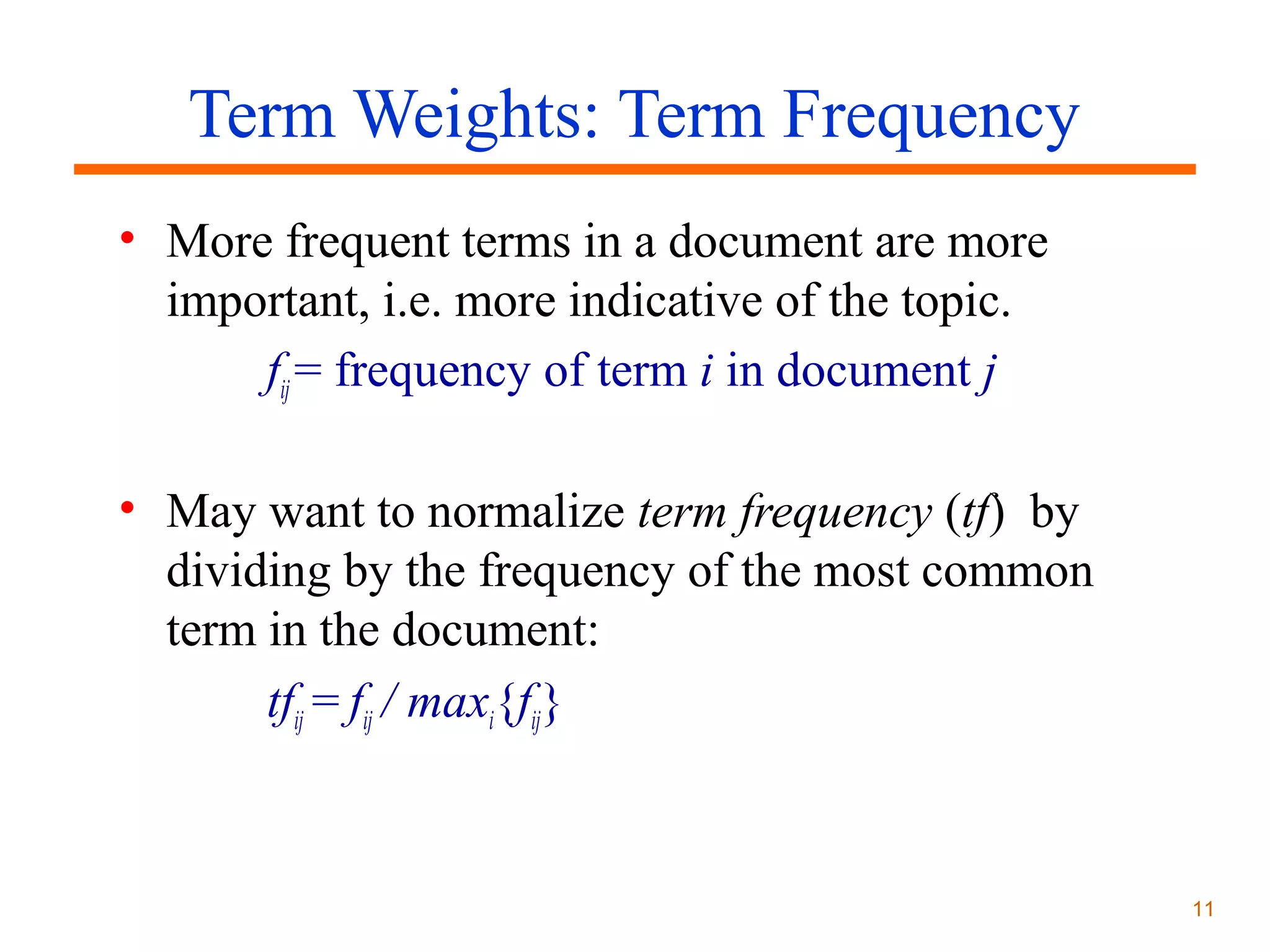
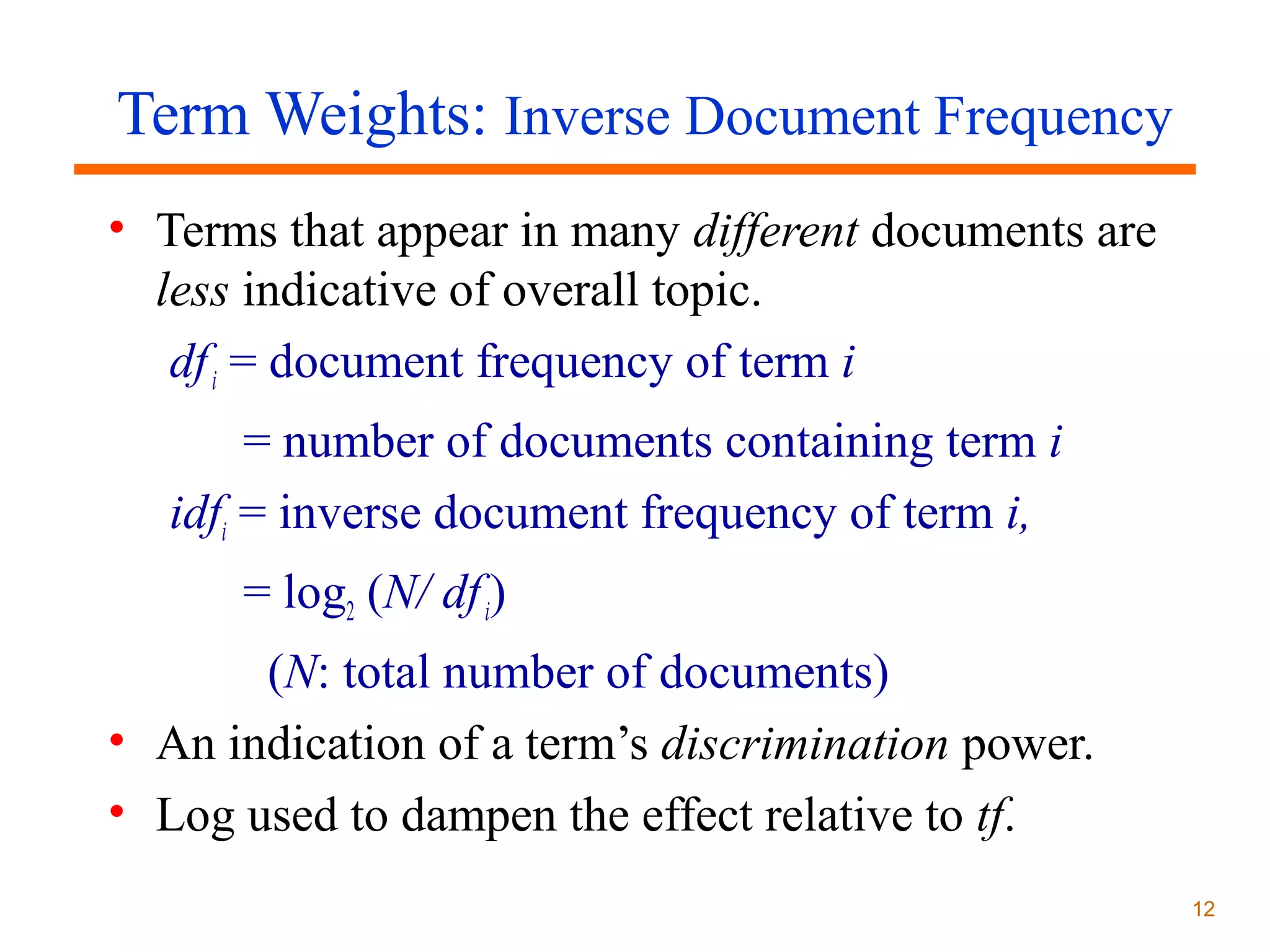
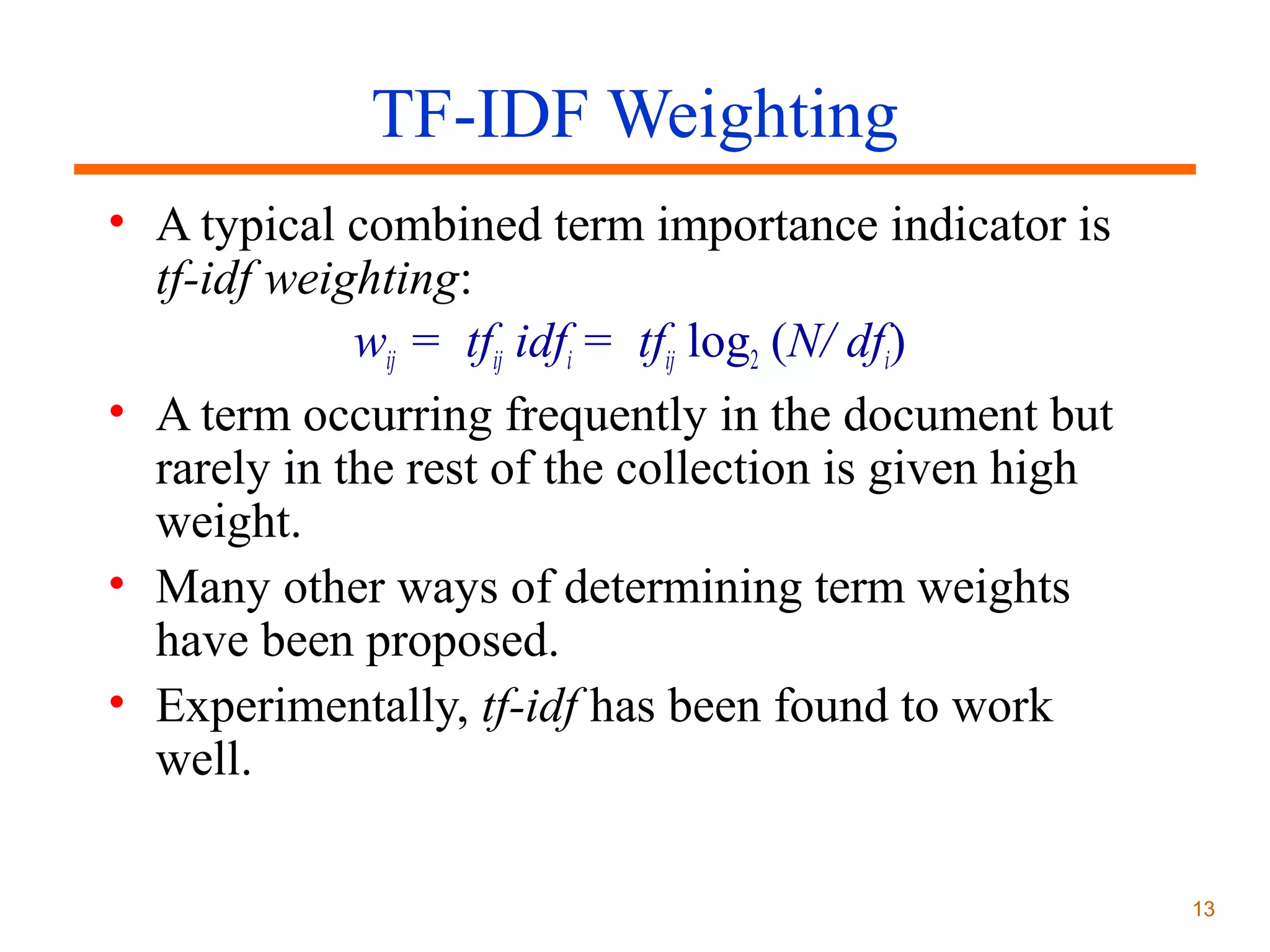
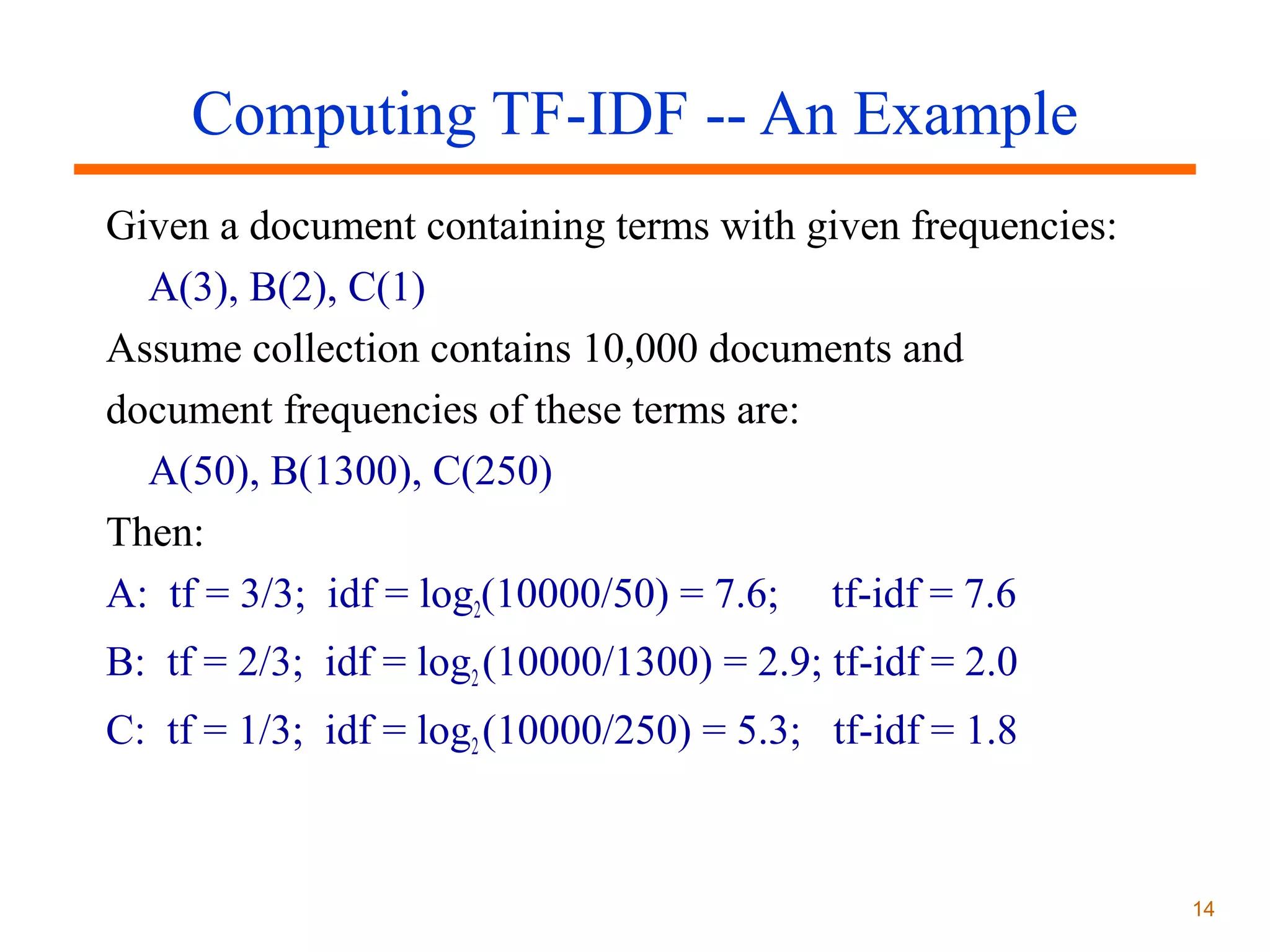
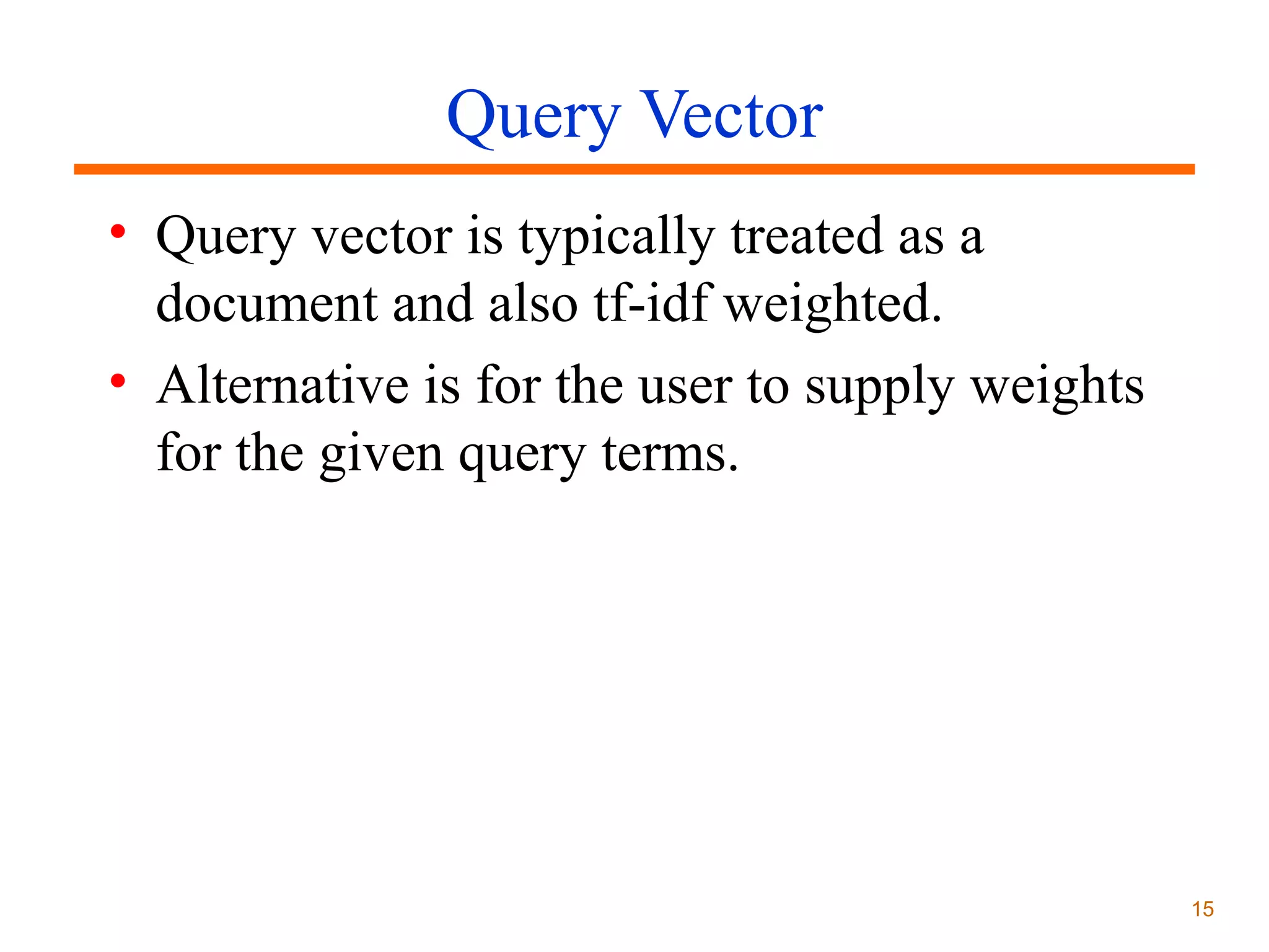
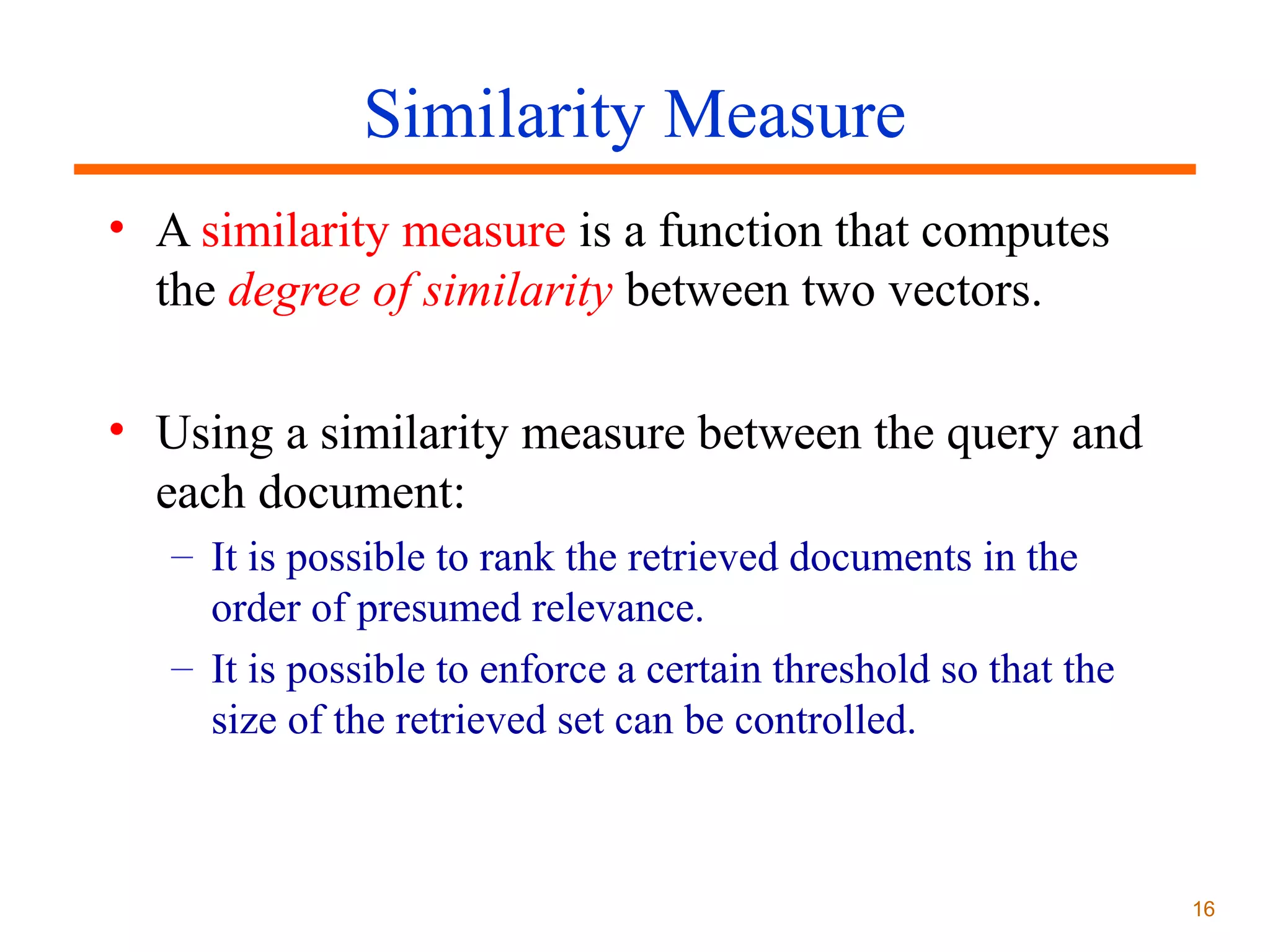
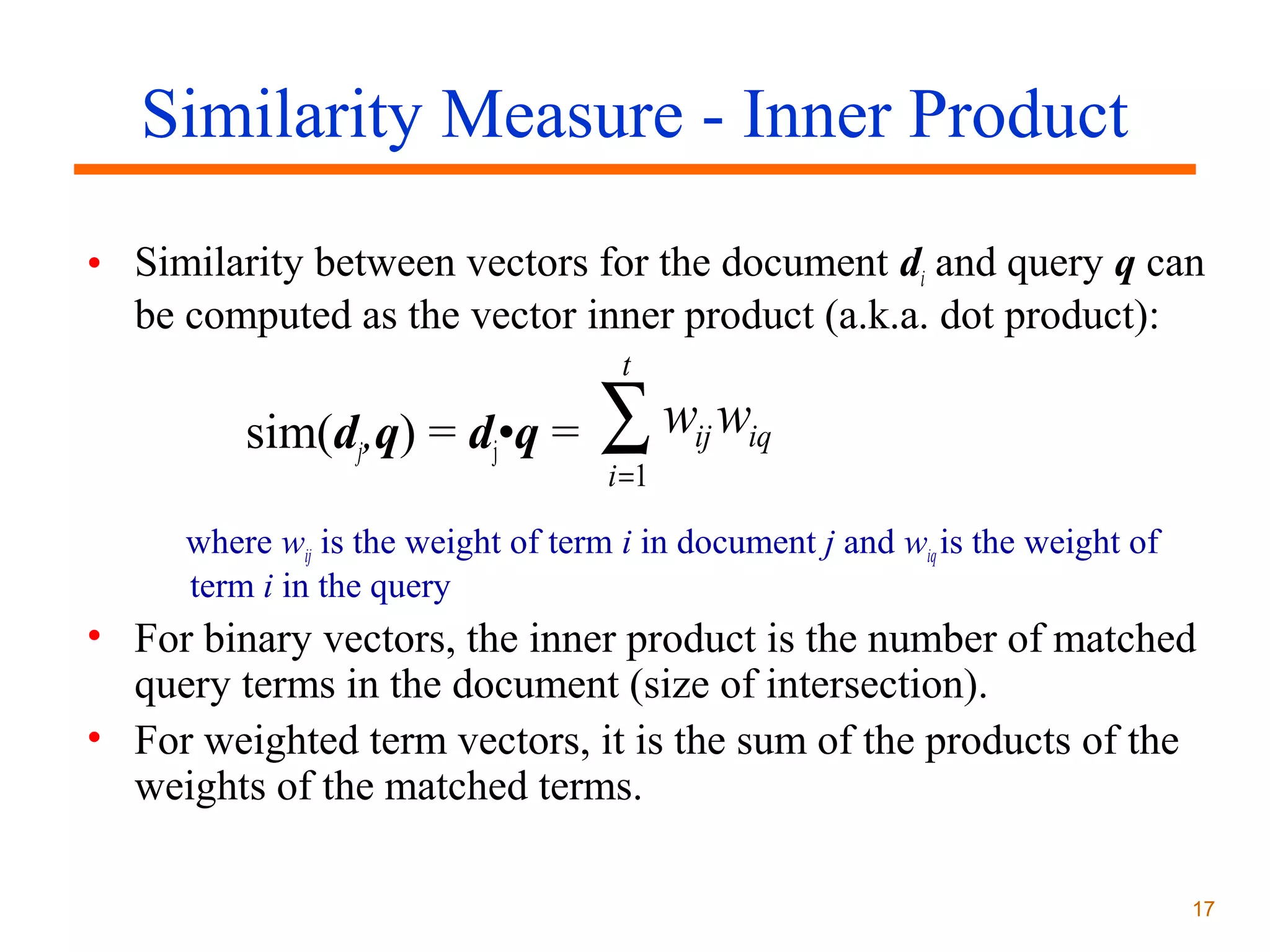
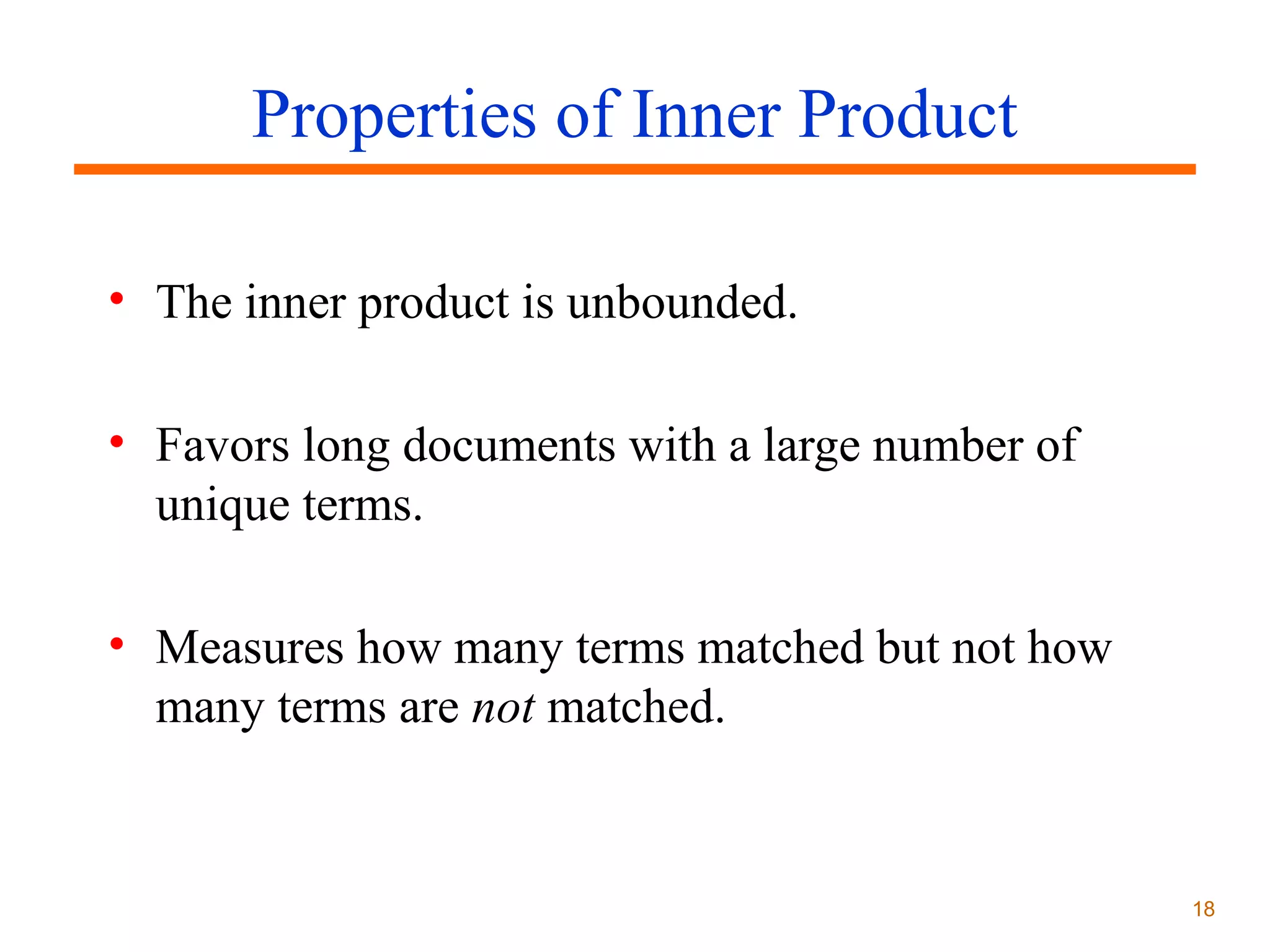
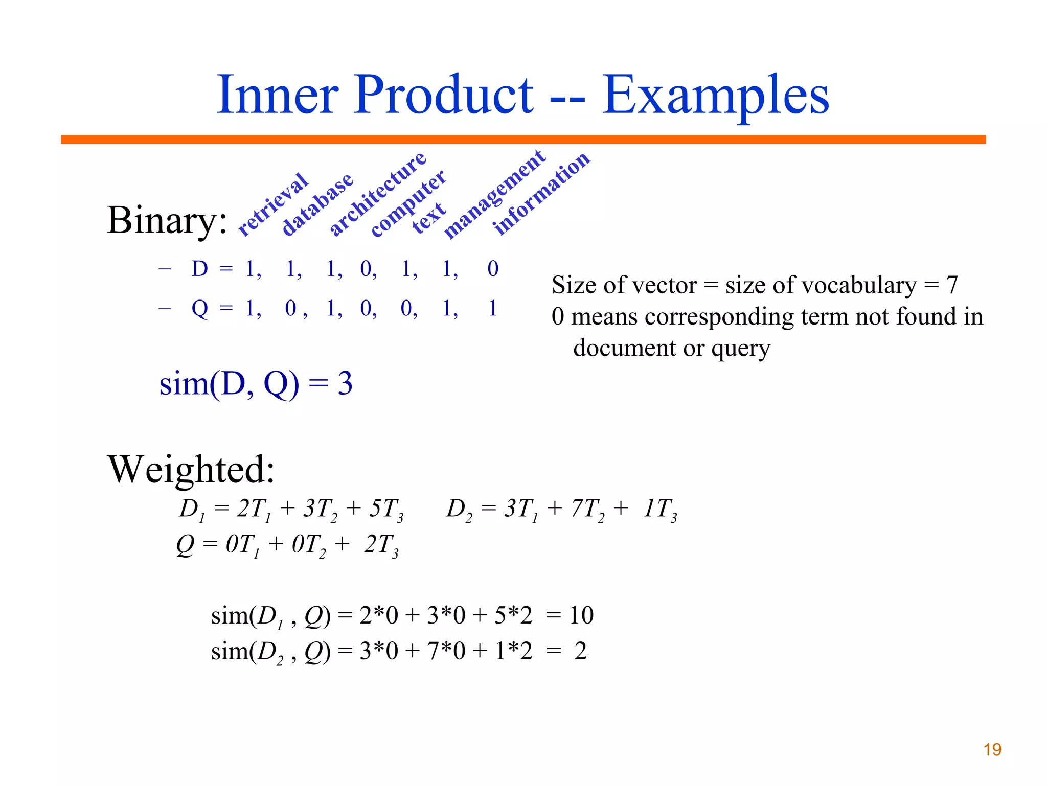
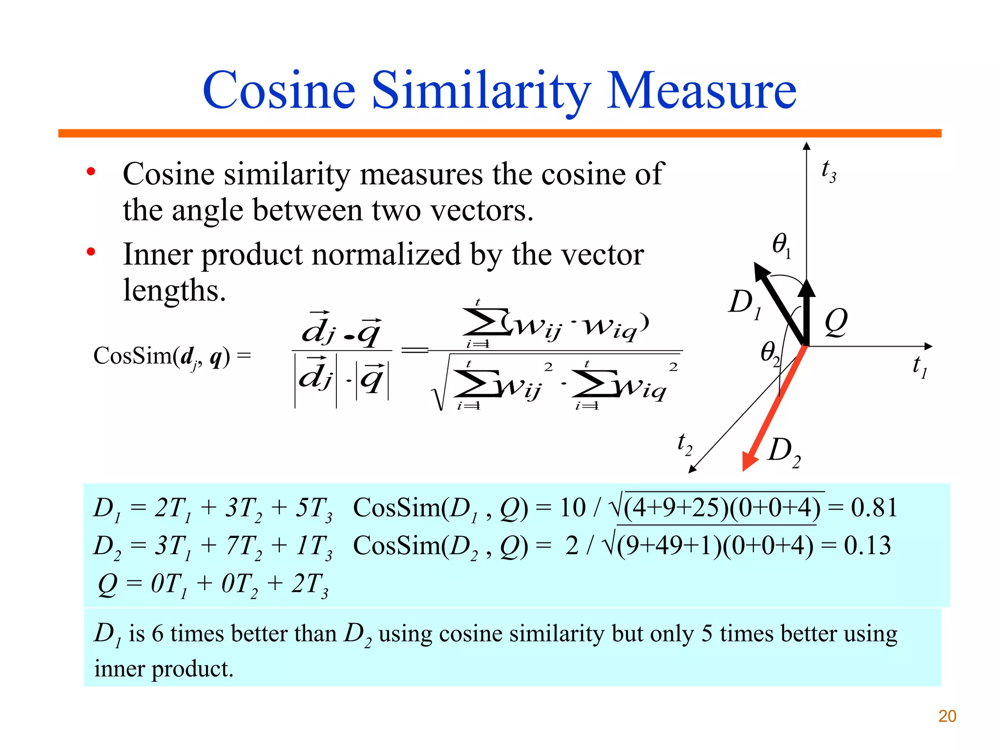
Boolean and Vector Space
Retrieval Models

1
Retrieval Models
• A retrieval model specifies the details
of:
– Document representation
– Query representation
– Retrieval function

• Determines a notion of relevance.
• Notion of relevance can be binary or
continuous (i.e. ranked retrieval).
2
Classes of Retrieval Models
• Boolean models (set theoretic)
– Extended Boolean

• Vector space models
(statistical/algebraic)
– Generalized VS
– Latent Semantic Indexing

• Probabilistic models
3
Common Preprocessing Steps
• Strip unwanted characters/markup (e.g. HTML
tags, punctuation, numbers, etc.).
• Break into tokens (keywords) on whitespace.
• Stem tokens to “root” words
– computational  comput

• Remove common stopwords (e.g. a, the, it, etc.).
• Detect common phrases (possibly using a domain
specific dictionary).
• Build inverted index (keyword  list of docs
containing it).
4
Statistical Models
• A document is typically represented by a bag of
words (unordered words with frequencies).
• Bag = set that allows multiple occurrences of the
same element.
• User specifies a set of desired terms with optional
weights:
– Weighted query terms:
Q = < database 0.5; text 0.8; information 0.2 >
– Unweighted query terms:
Q = < database; text; information >
– No Boolean conditions specified in the query.
5
Statistical Retrieval
• Retrieval based on similarity between query
and documents.
• Output documents are ranked according to
similarity to query.
• Similarity based on occurrence frequencies of
keywords in query and document.
• Automatic relevance feedback can be
supported:
– Relevant documents “added” to query.
– Irrelevant documents “subtracted” from query.

6
Issues for Vector Space Model
• How to determine important words in a
document?
– Word sense?
– Word n-grams (and phrases, idioms,…)  terms

• How to determine the degree of importance of a
term within a document and within the entire
collection?
• How to determine the degree of similarity between
a document and the query?
• In the case of the web, what is a collection and
what are the effects of links, formatting
information, etc.?
7
The Vector-Space Model
• Assume t distinct terms remain after
preprocessing; call them index terms or the
vocabulary.
• These “orthogonal” terms form a vector space.
Dimension = t = |vocabulary|

• Each term, i, in a document or query, j, is given a
real-valued weight, wij.
• Both documents and queries are expressed as
t-dimensional vectors:
dj = (w1j, w2j, …, wtj)
8
Graphic Representation
Example:
D1 = 2T1 + 3T2 + 5T3

T3

D2 = 3T1 + 7T2 + T3

5

Q = 0T1 + 0T2 + 2T3
D1 = 2T1+ 3T2 + 5T3

Q = 0T1 + 0T2 + 2T3
2

3

T1
D2 = 3T1 + 7T2 + T3

T2

7

3

• Is D1 or D2 more similar to Q?
• How to measure the degree of
similarity? Distance? Angle?
Projection?
9
Document Collection
• A collection of n documents can be represented in the
vector space model by a term-document matrix.
• An entry in the matrix corresponds to the “weight” of a
term in the document; zero means the term has no
significance in the document or it simply doesn’t exist in
the document.
T1 T2 ….
Tt
D1 w11 w21 …
wt1
D2 w12 w22 … wt2
:
:
:
:
:
:
:
:
Dn w1n w2n …
wtn
10
Term Weights: Term Frequency
• More frequent terms in a document are more
important, i.e. more indicative of the topic.
fij = frequency of term i in document j
• May want to normalize term frequency (tf) by
dividing by the frequency of the most common
term in the document:
tfij = fij / maxi{fij}

11
Term Weights: Inverse Document Frequency
• Terms that appear in many different documents are
less indicative of overall topic.
df i = document frequency of term i
= number of documents containing term i
idfi = inverse document frequency of term i,
= log2 (N/ df i)
(N: total number of documents)
• An indication of a term’s discrimination power.
• Log used to dampen the effect relative to tf.
12
TF-IDF Weighting
• A typical combined term importance indicator is
tf-idf weighting:
wij = tfij idfi = tfij log2 (N/ dfi)
• A term occurring frequently in the document but
rarely in the rest of the collection is given high
weight.
• Many other ways of determining term weights
have been proposed.
• Experimentally, tf-idf has been found to work
well.
13
Computing TF-IDF -- An Example
Given a document containing terms with given frequencies:
A(3), B(2), C(1)
Assume collection contains 10,000 documents and
document frequencies of these terms are:
A(50), B(1300), C(250)
Then:
A: tf = 3/3; idf = log2(10000/50) = 7.6; tf-idf = 7.6
B: tf = 2/3; idf = log2 (10000/1300) = 2.9; tf-idf = 2.0
C: tf = 1/3; idf = log2 (10000/250) = 5.3; tf-idf = 1.8

14
Query Vector
• Query vector is typically treated as a
document and also tf-idf weighted.
• Alternative is for the user to supply weights
for the given query terms.

15
Similarity Measure
• A similarity measure is a function that computes
the degree of similarity between two vectors.
• Using a similarity measure between the query and
each document:
– It is possible to rank the retrieved documents in the
order of presumed relevance.
– It is possible to enforce a certain threshold so that the
size of the retrieved set can be controlled.

16
Similarity Measure - Inner Product
• Similarity between vectors for the document di and query q can
be computed as the vector inner product (a.k.a. dot product):
t

sim(dj,q) = dj•q =

∑w w
i =1

ij

iq

where wij is the weight of term i in document j and wiq is the weight of
term i in the query

• For binary vectors, the inner product is the number of matched
query terms in the document (size of intersection).
• For weighted term vectors, it is the sum of the products of the
weights of the matched terms.
17
Properties of Inner Product
• The inner product is unbounded.
• Favors long documents with a large number of
unique terms.
• Measures how many terms matched but not how
many terms are not matched.

18
Inner Product -- Examples
Binary:

t
e
e n t io n
ur er
m a
al se ct t
ge rm
ev aba hite pu t
a o
i
etr dat arc com tex man inf
r

– D = 1, 1, 1, 0, 1, 1,

0

– Q = 1, 0 , 1, 0, 0, 1,

1

Size of vector = size of vocabulary = 7
0 means corresponding term not found in
document or query

sim(D, Q) = 3

Weighted:
D1 = 2T1 + 3T2 + 5T3
Q = 0T1 + 0T2 + 2T3

D2 = 3T1 + 7T2 + 1T3

sim(D1 , Q) = 2*0 + 3*0 + 5*2 = 10
sim(D2 , Q) = 3*0 + 7*0 + 1*2 = 2

19
Cosine Similarity Measure
• Cosine similarity measures the cosine of
the angle between two vectors.
• Inner product normalized by the vector
lengths.
 
(
dj q = ∑wij ⋅wiq )
 
CosSim(dj, q) =
dj ⋅ q
∑ ij ⋅∑ iq
w
w

t3

θ1

D1

t

•

i=
1

t

i=
1

2

t

2

θ2

Q
t1

i=
1

t2

D2

D1 = 2T1 + 3T2 + 5T3 CosSim(D1 , Q) = 10 / √(4+9+25)(0+0+4) = 0.81
D2 = 3T1 + 7T2 + 1T3 CosSim(D2 , Q) = 2 / √(9+49+1)(0+0+4) = 0.13
Q = 0T1 + 0T2 + 2T3
D1 is 6 times better than D2 using cosine similarity but only 5 times better using
inner product.
20
Comments on Vector Space Models
• Simple, mathematically based approach.
• Considers both local (tf) and global (idf) word
occurrence frequencies.
• Provides partial matching and ranked results.
• Tends to work quite well in practice despite
obvious weaknesses.
• Allows efficient implementation for large
document collections.

21

Ir models

  • 1.
    Boolean and VectorSpace Retrieval Models 1
  • 2.
    Retrieval Models • Aretrieval model specifies the details of: – Document representation – Query representation – Retrieval function • Determines a notion of relevance. • Notion of relevance can be binary or continuous (i.e. ranked retrieval). 2
  • 3.
    Classes of RetrievalModels • Boolean models (set theoretic) – Extended Boolean • Vector space models (statistical/algebraic) – Generalized VS – Latent Semantic Indexing • Probabilistic models 3
  • 4.
    Common Preprocessing Steps •Strip unwanted characters/markup (e.g. HTML tags, punctuation, numbers, etc.). • Break into tokens (keywords) on whitespace. • Stem tokens to “root” words – computational  comput • Remove common stopwords (e.g. a, the, it, etc.). • Detect common phrases (possibly using a domain specific dictionary). • Build inverted index (keyword  list of docs containing it). 4
  • 5.
    Statistical Models • Adocument is typically represented by a bag of words (unordered words with frequencies). • Bag = set that allows multiple occurrences of the same element. • User specifies a set of desired terms with optional weights: – Weighted query terms: Q = < database 0.5; text 0.8; information 0.2 > – Unweighted query terms: Q = < database; text; information > – No Boolean conditions specified in the query. 5
  • 6.
    Statistical Retrieval • Retrievalbased on similarity between query and documents. • Output documents are ranked according to similarity to query. • Similarity based on occurrence frequencies of keywords in query and document. • Automatic relevance feedback can be supported: – Relevant documents “added” to query. – Irrelevant documents “subtracted” from query. 6
  • 7.
    Issues for VectorSpace Model • How to determine important words in a document? – Word sense? – Word n-grams (and phrases, idioms,…)  terms • How to determine the degree of importance of a term within a document and within the entire collection? • How to determine the degree of similarity between a document and the query? • In the case of the web, what is a collection and what are the effects of links, formatting information, etc.? 7
  • 8.
    The Vector-Space Model •Assume t distinct terms remain after preprocessing; call them index terms or the vocabulary. • These “orthogonal” terms form a vector space. Dimension = t = |vocabulary| • Each term, i, in a document or query, j, is given a real-valued weight, wij. • Both documents and queries are expressed as t-dimensional vectors: dj = (w1j, w2j, …, wtj) 8
  • 9.
    Graphic Representation Example: D1 =2T1 + 3T2 + 5T3 T3 D2 = 3T1 + 7T2 + T3 5 Q = 0T1 + 0T2 + 2T3 D1 = 2T1+ 3T2 + 5T3 Q = 0T1 + 0T2 + 2T3 2 3 T1 D2 = 3T1 + 7T2 + T3 T2 7 3 • Is D1 or D2 more similar to Q? • How to measure the degree of similarity? Distance? Angle? Projection? 9
  • 10.
    Document Collection • Acollection of n documents can be represented in the vector space model by a term-document matrix. • An entry in the matrix corresponds to the “weight” of a term in the document; zero means the term has no significance in the document or it simply doesn’t exist in the document. T1 T2 …. Tt D1 w11 w21 … wt1 D2 w12 w22 … wt2 : : : : : : : : Dn w1n w2n … wtn 10
  • 11.
    Term Weights: TermFrequency • More frequent terms in a document are more important, i.e. more indicative of the topic. fij = frequency of term i in document j • May want to normalize term frequency (tf) by dividing by the frequency of the most common term in the document: tfij = fij / maxi{fij} 11
  • 12.
    Term Weights: InverseDocument Frequency • Terms that appear in many different documents are less indicative of overall topic. df i = document frequency of term i = number of documents containing term i idfi = inverse document frequency of term i, = log2 (N/ df i) (N: total number of documents) • An indication of a term’s discrimination power. • Log used to dampen the effect relative to tf. 12
  • 13.
    TF-IDF Weighting • Atypical combined term importance indicator is tf-idf weighting: wij = tfij idfi = tfij log2 (N/ dfi) • A term occurring frequently in the document but rarely in the rest of the collection is given high weight. • Many other ways of determining term weights have been proposed. • Experimentally, tf-idf has been found to work well. 13
  • 14.
    Computing TF-IDF --An Example Given a document containing terms with given frequencies: A(3), B(2), C(1) Assume collection contains 10,000 documents and document frequencies of these terms are: A(50), B(1300), C(250) Then: A: tf = 3/3; idf = log2(10000/50) = 7.6; tf-idf = 7.6 B: tf = 2/3; idf = log2 (10000/1300) = 2.9; tf-idf = 2.0 C: tf = 1/3; idf = log2 (10000/250) = 5.3; tf-idf = 1.8 14
  • 15.
    Query Vector • Queryvector is typically treated as a document and also tf-idf weighted. • Alternative is for the user to supply weights for the given query terms. 15
  • 16.
    Similarity Measure • Asimilarity measure is a function that computes the degree of similarity between two vectors. • Using a similarity measure between the query and each document: – It is possible to rank the retrieved documents in the order of presumed relevance. – It is possible to enforce a certain threshold so that the size of the retrieved set can be controlled. 16
  • 17.
    Similarity Measure -Inner Product • Similarity between vectors for the document di and query q can be computed as the vector inner product (a.k.a. dot product): t sim(dj,q) = dj•q = ∑w w i =1 ij iq where wij is the weight of term i in document j and wiq is the weight of term i in the query • For binary vectors, the inner product is the number of matched query terms in the document (size of intersection). • For weighted term vectors, it is the sum of the products of the weights of the matched terms. 17
  • 18.
    Properties of InnerProduct • The inner product is unbounded. • Favors long documents with a large number of unique terms. • Measures how many terms matched but not how many terms are not matched. 18
  • 19.
    Inner Product --Examples Binary: t e e n t io n ur er m a al se ct t ge rm ev aba hite pu t a o i etr dat arc com tex man inf r – D = 1, 1, 1, 0, 1, 1, 0 – Q = 1, 0 , 1, 0, 0, 1, 1 Size of vector = size of vocabulary = 7 0 means corresponding term not found in document or query sim(D, Q) = 3 Weighted: D1 = 2T1 + 3T2 + 5T3 Q = 0T1 + 0T2 + 2T3 D2 = 3T1 + 7T2 + 1T3 sim(D1 , Q) = 2*0 + 3*0 + 5*2 = 10 sim(D2 , Q) = 3*0 + 7*0 + 1*2 = 2 19
  • 20.
    Cosine Similarity Measure •Cosine similarity measures the cosine of the angle between two vectors. • Inner product normalized by the vector lengths.   ( dj q = ∑wij ⋅wiq )   CosSim(dj, q) = dj ⋅ q ∑ ij ⋅∑ iq w w t3 θ1 D1 t • i= 1 t i= 1 2 t 2 θ2 Q t1 i= 1 t2 D2 D1 = 2T1 + 3T2 + 5T3 CosSim(D1 , Q) = 10 / √(4+9+25)(0+0+4) = 0.81 D2 = 3T1 + 7T2 + 1T3 CosSim(D2 , Q) = 2 / √(9+49+1)(0+0+4) = 0.13 Q = 0T1 + 0T2 + 2T3 D1 is 6 times better than D2 using cosine similarity but only 5 times better using inner product. 20
  • 21.
    Comments on VectorSpace Models • Simple, mathematically based approach. • Considers both local (tf) and global (idf) word occurrence frequencies. • Provides partial matching and ranked results. • Tends to work quite well in practice despite obvious weaknesses. • Allows efficient implementation for large document collections. 21