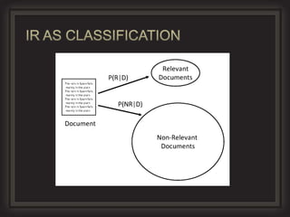
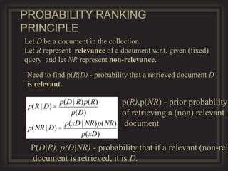
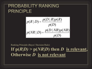
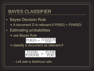
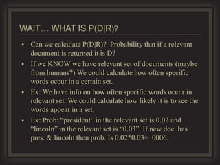
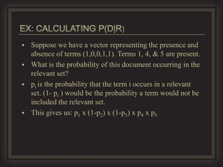
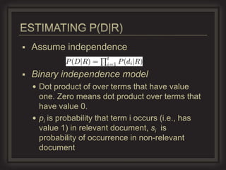
Probabilistic Retrieval Models
           Lecture 8
         Sean A. Golliher
   Need to quickly cover some old material
    to understand the new methods
   Complex concept that has been studied for
    some time
     Many factors to consider
     People often disagree when making relevance
     judgments
   Retrieval models make various assumptions
    about relevance to simplify problem
     e.g., topical vs. user relevance
     e.g., binary vs. multi-valued relevance
   Older models
     Boolean retrieval
     Vector Space model
   Probabilistic Models
     BM25
     Language models
   Combining evidence
     Inference networks
     Learning to Rank
   Two possible outcomes for query
    processing
     TRUE and FALSE
     “exact-match” retrieval
     simplest form of ranking
   Query usually specified using Boolean
    operators
     AND, OR, NOT
   Advantages
     Results are predictable, relatively easy to
      explain
     Many different features can be incorporated
     Efficient processing since many documents
      can be eliminated from search
   Disadvantages
     Effectiveness depends entirely on user
     Simple queries usually don’t work well
     Complex queries are difficult
 Documents and query represented by a
  vector of term weights
 Collection represented by a matrix of
  term weights
   3-d pictures useful, but can be
    misleading for high-dimensional space
The Euclidean
distance between q
and d2 is large even
though the
distribution of terms
in the query q and
the distribution of
terms in the
document d2 are
very similar.
   Thought experiment: take a document d and
    append it to itself. Call this document d′.
   “Semantically” d and d′ have the same content
   The Euclidean distance between the two
    documents can be quite large
   The angle between the two documents is 0,
    corresponding to maximal similarity (cos(0) = 1).
   Key idea: Rank documents according to angle with
    query.
 In Euclidean space, define dot product of
  vectors a & b as
ab=||a|| ||b|| cos               a


    where                             b
      ||a|| == length
         == angle between a & b
 By using Law of Cosines, can compute
  coordinate-dependent definition in 3-
  space:
 ab= axbx + ayby + azbz


 cos = ab/||a|| ||b||
 cosine(0) = 1
 cosine(90 deg) = 0
   Documents ranked by distance between
    points representing query and documents
     Similarity measure more common than a
      distance or dissimilarity measure
     e.g. Cosine correlation
 Consider two documents D1, D2 and a query
 Q
 ○ D1 = (0.5, 0.8, 0.3), D2 = (0.9, 0.4, 0.2), Q = (1.5, 1.0, 0)
Dot product         Unit vectors

                                            V
                 q    d    q   d                  q di
                                                i 1 i
    cos(q, d )                
                   q    d    q   d          V   2
                                                q
                                                           V
                                                                 d i2
                                            i 1 i          i   1


qi is the tf-idf weight of term i in the query
di is the tf-idf weight of term i in the document
cos(q,d) is the cosine similarity of q and d … or,
equivalently, the cosine of the angle between q and d.
   tf.idf weight (older retrieval model)
     tf: term frequency of term over collection of
      documents
     idf: inverse document freq. ex:
      ○ log(N/n)
          N is the total number of document
          n is total number of documents that contain a term
          Measure of “importance” of term. The more documents a
           term appears in the lest discriminating the term is.
          Use log to dampen the effects
     The collection frequency of t is the
      number of occurrences of t in the
      collection, counting multiple occurrences.
          Word   Collection frequency   Document frequency

    insurance                  10440                    3997
    try                        10422                    8760


 Document frequency df is number of
  documents that contain a term t.
 Which of these is more useful?
   The tf-idf weight of a term is the product of its
    tf weight and its idf weight.


   Best known weighting scheme in information retrieval
       ○ Note: the “-” in tf-idf is a hyphen, not a minus sign!
       ○ Alternative names: tf.idf, tf x idf
   Increases with the number of occurrences within a
    document
   Increases with the rarity of the term in the collection
 Rocchio algorithm (paper topic)
 Optimal query
     Maximizes the difference between the average
     vector representing the relevant documents and
     the average vector representing the non-relevant
     documents
   Modifies query according to

     α, β, and γ are parameters
      ○ Typical values 8, 16, 4
   Most dominant paradigm used today

   Probability theory is a strong foundation
    for representing uncertainty that is
    inherent in IR process.
   Robertson (1977)
    If a reference retrieval system’s response to each
    request is a ranking of the documents in the
    collection in order of decreasing probability of
    relevance to the user who submitted the request,
    where the probabilities are estimated as
    accurately as possible on the basis of whatever
    data have been made available to the system for
    this purpose, the overall effectiveness of the
    system to its user will be the best that is obtainable
    on the basis of those data.”
   Probability Ranking Principle (Robertson, 70ies;
    Maron, Kuhns, 1959)
   Information Retrieval as Probabilistic Inference
    (van Rijsbergen & co, since 70ies)
   Probabilistic Indexing (Fuhr & Co.,late 80ies-
    90ies)
   Bayesian Nets in IR (Turtle, Croft, 90ies)
   Probabilistic Logic Programming in IR (Fuhr &
    co, 90ies)
   P(a | b) => Conditional probability. Probability of a given
    that b occurred.
   Basic definitions


    (a È b) => AorB
    (a Ç b) = AandB
Let a, b be two events.

  p(a | b)p(b) = p(a Ç b) = p(b | a)p(a)
             p(b | a)p(a)
  p(a | b) =
                p(b)
  p(a | b)p(b) = p(b | a)p(a)
   Let D be a document in the collection.
   Let R represent relevance of a document w.r.t. given
    (fixed) query and let NR represent non-relevance.
   How do we find P(R|D)? Probability that a retrieved
    document is relevant. Abstract concept.
   P(R) is the probability that a retrieved is relevant
   Not Clear how to calculate this.
   Can we calculate P(D|R)? Probability of a document
    occurring in a set given a relevant set has been returned.
   If we KNOW we have relevant set of documents (maybe
    from humans?) We could calculate how often specific
    words occur in a certain set.
Let D be a document in the collection.
Let R represent relevance of a document w.r.t. given (fixed)
query and let NR represent non-relevance.

Need to find p(R|D) - probability that a retrieved document D
is relevant.

           p(D | R)p(R)      p(R),p(NR) - prior probability
 p(R | D) =
               p(D)          of retrieving a (non) relevant
             p(xD | NR)p(NR) document
 p(NR | D) =
                  p(xD)
  P(D|R), p(D|NR) - probability that if a relevant (non-rel
  document is retrieved, it is D.
p(D | R)p(R)
                p(R | D) =
                              p(D)
                            p(D | NR)p(NR)
                p(NR | D) =
                                  p(D)

Ranking Principle (Bayes’ Decision Rule):

If p(R|D) > p(NR|D) then D is relevant,
Otherwise D is not relevant
   Bayes Decision Rule
     A document D is relevant if P(R|D) > P(NR|D)
   Estimating probabilities
     use Bayes Rule


     classify a document as relevant if


      ○ Left side is likelihood ratio
   Can we calculate P(D|R)? Probability that if a relevant
    document is returned it is D?
   If we KNOW we have relevant set of documents (maybe
    from humans?) We could calculate how often specific
    words occur in a certain set.
   Ex: We have info on how often specific words occur in
    relevant set. We could calculate how likely it is to see the
    words appear in a set.
   Ex: Prob: “president” in the relevant set is 0.02 and
    “lincoln” in the relevant set is “0.03”. If new doc. has
    pres. & lincoln then prob. Is 0.02*0.03= .0006.
   Suppose we have a vector representing the presence and
    absence of terms (1,0,0,1,1). Terms 1, 4, & 5 are present.
   What is the probability of this document occurring in the
    relevant set?
   pi is the probability that the term i occurs in a relevant
    set. (1- pi ) would be the probability a term would not be
    included the relevant set.
   This gives us: p1 x (1-p2) x (1-p3) x p4 x p5
   Assume independence

   Binary independence model
     Dot product of over terms that have value
      one. Zero means dot product over terms that
      have value 0.
     pi is probability that term i occurs (i.e., has
      value 1) in relevant document, si is
      probability of occurrence in non-relevant
      document
   Scoring function is (Last term was same
    for all documents. So it can be ignored.
 Jump to machine learning and web
  search. Lots of training data available
  from web search queries. Learning to
  rank models.
 http://www.bradblock.com/A_General_La
  nguage_Model_for_Information_Retrieval
  .pdf

Probabilistic Retrieval Models - Sean Golliher Lecture 8 MSU CSCI 494

  • 1.
    Probabilistic Retrieval Models Lecture 8 Sean A. Golliher
  • 2.
    Need to quickly cover some old material to understand the new methods
  • 3.
    Complex concept that has been studied for some time  Many factors to consider  People often disagree when making relevance judgments  Retrieval models make various assumptions about relevance to simplify problem  e.g., topical vs. user relevance  e.g., binary vs. multi-valued relevance
  • 4.
    Older models  Boolean retrieval  Vector Space model  Probabilistic Models  BM25  Language models  Combining evidence  Inference networks  Learning to Rank
  • 5.
    Two possible outcomes for query processing  TRUE and FALSE  “exact-match” retrieval  simplest form of ranking  Query usually specified using Boolean operators  AND, OR, NOT
  • 6.
    Advantages  Results are predictable, relatively easy to explain  Many different features can be incorporated  Efficient processing since many documents can be eliminated from search  Disadvantages  Effectiveness depends entirely on user  Simple queries usually don’t work well  Complex queries are difficult
  • 7.
     Documents andquery represented by a vector of term weights  Collection represented by a matrix of term weights
  • 9.
    3-d pictures useful, but can be misleading for high-dimensional space
  • 10.
    The Euclidean distance betweenq and d2 is large even though the distribution of terms in the query q and the distribution of terms in the document d2 are very similar.
  • 11.
    Thought experiment: take a document d and append it to itself. Call this document d′.  “Semantically” d and d′ have the same content  The Euclidean distance between the two documents can be quite large  The angle between the two documents is 0, corresponding to maximal similarity (cos(0) = 1).  Key idea: Rank documents according to angle with query.
  • 12.
     In Euclideanspace, define dot product of vectors a & b as ab=||a|| ||b|| cos a where b ||a|| == length == angle between a & b
  • 13.
     By usingLaw of Cosines, can compute coordinate-dependent definition in 3- space:  ab= axbx + ayby + azbz  cos = ab/||a|| ||b||  cosine(0) = 1  cosine(90 deg) = 0
  • 14.
    Documents ranked by distance between points representing query and documents  Similarity measure more common than a distance or dissimilarity measure  e.g. Cosine correlation
  • 15.
     Consider twodocuments D1, D2 and a query Q ○ D1 = (0.5, 0.8, 0.3), D2 = (0.9, 0.4, 0.2), Q = (1.5, 1.0, 0)
  • 16.
    Dot product Unit vectors     V   q d q d q di i 1 i cos(q, d )     q d q d V 2 q V d i2 i 1 i i 1 qi is the tf-idf weight of term i in the query di is the tf-idf weight of term i in the document cos(q,d) is the cosine similarity of q and d … or, equivalently, the cosine of the angle between q and d.
  • 17.
    tf.idf weight (older retrieval model)  tf: term frequency of term over collection of documents  idf: inverse document freq. ex: ○ log(N/n)  N is the total number of document  n is total number of documents that contain a term  Measure of “importance” of term. The more documents a term appears in the lest discriminating the term is.  Use log to dampen the effects
  • 18.
    The collection frequency of t is the number of occurrences of t in the collection, counting multiple occurrences. Word Collection frequency Document frequency insurance 10440 3997 try 10422 8760  Document frequency df is number of documents that contain a term t.  Which of these is more useful?
  • 19.
    The tf-idf weight of a term is the product of its tf weight and its idf weight.  Best known weighting scheme in information retrieval ○ Note: the “-” in tf-idf is a hyphen, not a minus sign! ○ Alternative names: tf.idf, tf x idf  Increases with the number of occurrences within a document  Increases with the rarity of the term in the collection
  • 20.
     Rocchio algorithm(paper topic)  Optimal query  Maximizes the difference between the average vector representing the relevant documents and the average vector representing the non-relevant documents  Modifies query according to  α, β, and γ are parameters ○ Typical values 8, 16, 4
  • 21.
    Most dominant paradigm used today  Probability theory is a strong foundation for representing uncertainty that is inherent in IR process.
  • 22.
    Robertson (1977) If a reference retrieval system’s response to each request is a ranking of the documents in the collection in order of decreasing probability of relevance to the user who submitted the request, where the probabilities are estimated as accurately as possible on the basis of whatever data have been made available to the system for this purpose, the overall effectiveness of the system to its user will be the best that is obtainable on the basis of those data.”
  • 23.
    Probability Ranking Principle (Robertson, 70ies; Maron, Kuhns, 1959)  Information Retrieval as Probabilistic Inference (van Rijsbergen & co, since 70ies)  Probabilistic Indexing (Fuhr & Co.,late 80ies- 90ies)  Bayesian Nets in IR (Turtle, Croft, 90ies)  Probabilistic Logic Programming in IR (Fuhr & co, 90ies)
  • 24.
    P(a | b) => Conditional probability. Probability of a given that b occurred.  Basic definitions (a È b) => AorB (a Ç b) = AandB
  • 25.
    Let a, bbe two events. p(a | b)p(b) = p(a Ç b) = p(b | a)p(a) p(b | a)p(a) p(a | b) = p(b) p(a | b)p(b) = p(b | a)p(a)
  • 26.
    Let D be a document in the collection.  Let R represent relevance of a document w.r.t. given (fixed) query and let NR represent non-relevance.  How do we find P(R|D)? Probability that a retrieved document is relevant. Abstract concept.  P(R) is the probability that a retrieved is relevant  Not Clear how to calculate this.
  • 27.
    Can we calculate P(D|R)? Probability of a document occurring in a set given a relevant set has been returned.  If we KNOW we have relevant set of documents (maybe from humans?) We could calculate how often specific words occur in a certain set.
  • 29.
    Let D bea document in the collection. Let R represent relevance of a document w.r.t. given (fixed) query and let NR represent non-relevance. Need to find p(R|D) - probability that a retrieved document D is relevant. p(D | R)p(R) p(R),p(NR) - prior probability p(R | D) = p(D) of retrieving a (non) relevant p(xD | NR)p(NR) document p(NR | D) = p(xD) P(D|R), p(D|NR) - probability that if a relevant (non-rel document is retrieved, it is D.
  • 30.
    p(D | R)p(R) p(R | D) = p(D) p(D | NR)p(NR) p(NR | D) = p(D) Ranking Principle (Bayes’ Decision Rule): If p(R|D) > p(NR|D) then D is relevant, Otherwise D is not relevant
  • 31.
    Bayes Decision Rule  A document D is relevant if P(R|D) > P(NR|D)  Estimating probabilities  use Bayes Rule  classify a document as relevant if ○ Left side is likelihood ratio
  • 32.
    Can we calculate P(D|R)? Probability that if a relevant document is returned it is D?  If we KNOW we have relevant set of documents (maybe from humans?) We could calculate how often specific words occur in a certain set.  Ex: We have info on how often specific words occur in relevant set. We could calculate how likely it is to see the words appear in a set.  Ex: Prob: “president” in the relevant set is 0.02 and “lincoln” in the relevant set is “0.03”. If new doc. has pres. & lincoln then prob. Is 0.02*0.03= .0006.
  • 33.
    Suppose we have a vector representing the presence and absence of terms (1,0,0,1,1). Terms 1, 4, & 5 are present.  What is the probability of this document occurring in the relevant set?  pi is the probability that the term i occurs in a relevant set. (1- pi ) would be the probability a term would not be included the relevant set.  This gives us: p1 x (1-p2) x (1-p3) x p4 x p5
  • 34.
    Assume independence  Binary independence model  Dot product of over terms that have value one. Zero means dot product over terms that have value 0.  pi is probability that term i occurs (i.e., has value 1) in relevant document, si is probability of occurrence in non-relevant document
  • 36.
    Scoring function is (Last term was same for all documents. So it can be ignored.
  • 37.
     Jump tomachine learning and web search. Lots of training data available from web search queries. Learning to rank models.  http://www.bradblock.com/A_General_La nguage_Model_for_Information_Retrieval .pdf

Editor's Notes

  • #12 Angle captures relative proportion of terms
  • #19 http://nlp.stanford.edu/IR-book/html/htmledition/inverse-document-frequency-1.html … For example auto industry. All documents contain the word auto. Want to decrease the value of that phraseas it occurs more because it is non discriminating in a search query. Df is more useful.. Look at the range.
  • #20 Tf is the number of times the word occurs in document d.
  • #29 D is a collection of documents. R is relevance. P(R) Is
  • #37 Use log since we get lots of small numbers. pi is probablity that that term I occurs in relevant set.
  • #38 Use log since we get lots of small numbers. pi is probablity that that term I occurs in relevant set.