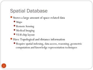
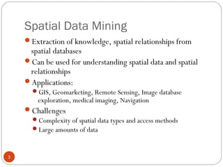
1
Spatial Data Mining
Spatial Database
2
Stores a large amount of space-related data
Maps
Remote Sensing
Medical Imaging
VLSI chip layout
Have Topological and distance information
Require spatial indexing, data access, reasoning ,geometric
computation and knowledge representation techniques
Spatial Data Mining
3
Extraction of knowledge, spatial relationships from
spatial databases
Can be used for understanding spatial data and spatial
relationships
Applications:
GIS, Geomarketing, Remote Sensing, Image database
exploration, medical imaging, Navigation
Challenges
Complexity of spatial data types and access methods
Large amounts of data
Cont.
4
Non-spatial Information
Same as data in traditional data mining
Numerical, categorical, ordinal, boolean, etc
e.g., city name, city population
Spatial Information
Spatial attribute: geographically referenced
 Neighborhood and extent
Location, e.g., longitude, latitude, elevation
Spatial data representations
Raster: gridded space
Vector: point, line, polygon
Graph: node, edge, path
Spatial Data
5
Cont.
6
Statistical techniques
7
Popular approach to analyze spatial data
Assumes independence among spatial data
Can be performed only by experts
Do not work well with symbolic values
Spatial Data Warehousing
8
Spatial data warehouse: Integrated, subject-oriented, time-variant,
and nonvolatile spatial data repository.
It consists of both spatial and non spatial in support of spatial data mining
and spatial-data-related decision-making processes.
Spatial data cube: multidimensional spatial database
Both dimensions and measures may contain spatial components.
Challenging issues:
Spatial data integration: a big issue
Structure-specific formats (raster- vs. vector-based, OO vs. relational models,
different storage and indexing, etc.)
Vendor-specific formats (ESRI, MapInfo, Intergraph, IDRISI, etc.)
Realization of Fast and flexible OLAP in spatial data warehouses.
Dimensions and Measures in Spatial
Data Warehouse
9
Dimensions
non-spatial
e.g. “25-30 degrees” generalizes to“hot” (both are strings)
spatial-to-non spatial
e.g. Seattle generalizes to description “Pacific Northwest” (as a string)
spatial-to-spatial
e.g. Seattle generalizes to Pacific Northwest (as a spatial region)
Measures
numerical (e.g. monthly revenue of a region)
distributive (e.g. count, sum)
algebraic (e.g. average)
holistic (e.g. median, rank)
spatial
collection of spatial pointers (e.g. pointers to all regions with temperature of
25-30 degrees in July)
Example: British Columbia Weather
Pattern Analysis
10
Input
A map with about 3,000 weather probes scattered in B.C.
Recording daily data for temperature, precipitation, wind velocity, etc. for a designated
small area and transmitting signal to a provincial weather station.
Data warehouse using star schema
Output
A map that reveals patterns: merged (similar) regions
Goals
Interactive analysis (drill-down, slice, dice, pivot, roll-up)
Fast response time
Minimizing storage space used
Challenge
A merged region may contain hundreds of “primitive” regions (polygons)
Star Schema of the BC Weather
Warehouse
Spatial data warehouse
Dimensions
region_name
time
temperature
precipitation
Measurements
region_map
area
count
11Fact tableDimension table
12
Can we precompute all of the possible spatial merges
and store them in the corresponding cuboid cells of a
spatial data cube?
Probably not.
It requires multi-megabytes of storage.
On-line computation is slow and expensive.
Dynamic Merging of Spatial
Objects
13
Methods for Computing Spatial Data
Cubes
14
On-line aggregation: collect and store pointers to spatial
objects in a spatial data cube
expensive and slow, need efficient aggregation techniques
Precompute and store all the possible combinations
huge space overhead
Precompute and store rough approximations in a spatial data
cube
accuracy trade-off, MBR
Selective computation: only materialize those which will be
accessed frequently
a reasonable choice
Mining Spatial Association and
Co-location Patterns
15
Spatial association rule: A ⇒ B [s%, c%]
A and B are sets of spatial or non-spatial predicates
Topological relations: intersects, overlaps, disjoint, etc.
Spatial orientations: left_of, west_of, under, etc.
Distance information: close_to, within_distance, etc.
s% is the support and c% is the confidence of the rule
Examples
is_a(x, “School”) ^ Close_to(x, “Sports_Center”) → close_to(x, “Park”)
[7%, 85%]
Progressive Refinement
16
Progressive Refinement:
spatial association mining needs to evaluate multiple spatial relationships
among a large no. of spatial object – expensive.
Hierarchy of spatial relationship:
First search for rough relationship and then refine it
Superset coverage property – all the potential answers should be perserved
(i.e.false-positive test).
Two-step mining of spatial association:
Step 1: Rough spatial computation (as a filter)
 Using MBR for rough estimation
Step2: Detailed spatial algorithm (as refinement)
 Apply only to those objects which have passed the rough spatial association test
(no less than min_support)
Spatial co-locations
17
Just what one really wants to explore.
Based on the property of spatial autocorrelation, interesting
features likely coexist in closely located regions.
Efficient methods - Apriori , progressive refinement,etc.
18
Spatial Cluster Analysis
19
• Mining clusters—k-means, k-medoids, hierarchical, density-based,
etc.
• Analysis of distinct features of the clusters
Spatial Classification
20
Analyze spatial objects to derive classification schemes, such
as decision trees, in relevance to certain spatial properties
(district, highway, river, etc.)
Classifying medium-size families according to income, region, and infant mortality
rates
Mining for volcanoes on Venus
Employ methods such as:
Decision-tree classification, Naïve-Bayesian classifier + boosting, neural network,
genetic programming, etc.
Spatial Trend Analysis
21
Function
Detect changes and trends along a spatial dimension
Study the trend of non-spatial or spatial data changing with space
Application examples
Observe the trend of changes of the climate or vegetation with
increasing distance from an ocean
Crime rate or unemployment rate change with regard to city geo-
distribution.
Traffic flows in highways and in cities.
Mining Raster Databases
22
Vector data Mining
Maps
Graphs
Molecular chains
Raster data mining
Satellite Images
23
Other Applications
24
Spatial data mining is used in
 NASA Earth Observing System (EOS): Earth science data
National Inst. of Justice: crime mapping
 Census Bureau, Dept. of Commerce: census data
 Dept. of Transportation (DOT): traffic data
National Inst. of Health(NIH): cancer clusters
 Commerce, e.g. Retail Analysis

4.2 spatial data mining

  • 1.
  • 2.
    Spatial Database 2 Stores alarge amount of space-related data Maps Remote Sensing Medical Imaging VLSI chip layout Have Topological and distance information Require spatial indexing, data access, reasoning ,geometric computation and knowledge representation techniques
  • 3.
    Spatial Data Mining 3 Extractionof knowledge, spatial relationships from spatial databases Can be used for understanding spatial data and spatial relationships Applications: GIS, Geomarketing, Remote Sensing, Image database exploration, medical imaging, Navigation Challenges Complexity of spatial data types and access methods Large amounts of data
  • 4.
    Cont. 4 Non-spatial Information Same asdata in traditional data mining Numerical, categorical, ordinal, boolean, etc e.g., city name, city population Spatial Information Spatial attribute: geographically referenced  Neighborhood and extent Location, e.g., longitude, latitude, elevation Spatial data representations Raster: gridded space Vector: point, line, polygon Graph: node, edge, path
  • 5.
  • 6.
  • 7.
    Statistical techniques 7 Popular approachto analyze spatial data Assumes independence among spatial data Can be performed only by experts Do not work well with symbolic values
  • 8.
    Spatial Data Warehousing 8 Spatialdata warehouse: Integrated, subject-oriented, time-variant, and nonvolatile spatial data repository. It consists of both spatial and non spatial in support of spatial data mining and spatial-data-related decision-making processes. Spatial data cube: multidimensional spatial database Both dimensions and measures may contain spatial components. Challenging issues: Spatial data integration: a big issue Structure-specific formats (raster- vs. vector-based, OO vs. relational models, different storage and indexing, etc.) Vendor-specific formats (ESRI, MapInfo, Intergraph, IDRISI, etc.) Realization of Fast and flexible OLAP in spatial data warehouses.
  • 9.
    Dimensions and Measuresin Spatial Data Warehouse 9 Dimensions non-spatial e.g. “25-30 degrees” generalizes to“hot” (both are strings) spatial-to-non spatial e.g. Seattle generalizes to description “Pacific Northwest” (as a string) spatial-to-spatial e.g. Seattle generalizes to Pacific Northwest (as a spatial region) Measures numerical (e.g. monthly revenue of a region) distributive (e.g. count, sum) algebraic (e.g. average) holistic (e.g. median, rank) spatial collection of spatial pointers (e.g. pointers to all regions with temperature of 25-30 degrees in July)
  • 10.
    Example: British ColumbiaWeather Pattern Analysis 10 Input A map with about 3,000 weather probes scattered in B.C. Recording daily data for temperature, precipitation, wind velocity, etc. for a designated small area and transmitting signal to a provincial weather station. Data warehouse using star schema Output A map that reveals patterns: merged (similar) regions Goals Interactive analysis (drill-down, slice, dice, pivot, roll-up) Fast response time Minimizing storage space used Challenge A merged region may contain hundreds of “primitive” regions (polygons)
  • 11.
    Star Schema ofthe BC Weather Warehouse Spatial data warehouse Dimensions region_name time temperature precipitation Measurements region_map area count 11Fact tableDimension table
  • 12.
    12 Can we precomputeall of the possible spatial merges and store them in the corresponding cuboid cells of a spatial data cube? Probably not. It requires multi-megabytes of storage. On-line computation is slow and expensive.
  • 13.
    Dynamic Merging ofSpatial Objects 13
  • 14.
    Methods for ComputingSpatial Data Cubes 14 On-line aggregation: collect and store pointers to spatial objects in a spatial data cube expensive and slow, need efficient aggregation techniques Precompute and store all the possible combinations huge space overhead Precompute and store rough approximations in a spatial data cube accuracy trade-off, MBR Selective computation: only materialize those which will be accessed frequently a reasonable choice
  • 15.
    Mining Spatial Associationand Co-location Patterns 15 Spatial association rule: A ⇒ B [s%, c%] A and B are sets of spatial or non-spatial predicates Topological relations: intersects, overlaps, disjoint, etc. Spatial orientations: left_of, west_of, under, etc. Distance information: close_to, within_distance, etc. s% is the support and c% is the confidence of the rule Examples is_a(x, “School”) ^ Close_to(x, “Sports_Center”) → close_to(x, “Park”) [7%, 85%]
  • 16.
    Progressive Refinement 16 Progressive Refinement: spatialassociation mining needs to evaluate multiple spatial relationships among a large no. of spatial object – expensive. Hierarchy of spatial relationship: First search for rough relationship and then refine it Superset coverage property – all the potential answers should be perserved (i.e.false-positive test). Two-step mining of spatial association: Step 1: Rough spatial computation (as a filter)  Using MBR for rough estimation Step2: Detailed spatial algorithm (as refinement)  Apply only to those objects which have passed the rough spatial association test (no less than min_support)
  • 17.
    Spatial co-locations 17 Just whatone really wants to explore. Based on the property of spatial autocorrelation, interesting features likely coexist in closely located regions. Efficient methods - Apriori , progressive refinement,etc.
  • 18.
  • 19.
    Spatial Cluster Analysis 19 •Mining clusters—k-means, k-medoids, hierarchical, density-based, etc. • Analysis of distinct features of the clusters
  • 20.
    Spatial Classification 20 Analyze spatialobjects to derive classification schemes, such as decision trees, in relevance to certain spatial properties (district, highway, river, etc.) Classifying medium-size families according to income, region, and infant mortality rates Mining for volcanoes on Venus Employ methods such as: Decision-tree classification, Naïve-Bayesian classifier + boosting, neural network, genetic programming, etc.
  • 21.
    Spatial Trend Analysis 21 Function Detectchanges and trends along a spatial dimension Study the trend of non-spatial or spatial data changing with space Application examples Observe the trend of changes of the climate or vegetation with increasing distance from an ocean Crime rate or unemployment rate change with regard to city geo- distribution. Traffic flows in highways and in cities.
  • 22.
    Mining Raster Databases 22 Vectordata Mining Maps Graphs Molecular chains Raster data mining Satellite Images
  • 23.
  • 24.
    Other Applications 24 Spatial datamining is used in  NASA Earth Observing System (EOS): Earth science data National Inst. of Justice: crime mapping  Census Bureau, Dept. of Commerce: census data  Dept. of Transportation (DOT): traffic data National Inst. of Health(NIH): cancer clusters  Commerce, e.g. Retail Analysis