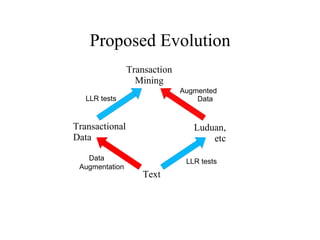
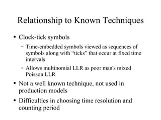
The document discusses using log-likelihood ratio (LLR) tests to analyze transactional data. It defines transactional data as sequences of transactions that may include symbols, times, and amounts. The document proposes applying LLR tests to transactional data by decomposing the LLR test into terms for symbols/timing and amounts. Examples of applying this methodology to problems in insurance risk prediction, fraud detection, and system monitoring are provided.

1. Mining Transactional Data
Ted Dunning - 2004

2. Outline
● What are LLR tests?
– What value have they shown?
● What are transactional values?
– How can we define LLR tests for them?
● How can these methods be applied?
– Modeling architecture examples
● How new is this?

3. Log-likelihood Ratio Tests
● Theorem due to Chernoff showed that
generalized log-likelihood ratio is asymptotically
2 distributed in many useful cases
● Most well known statistical tests are either
approximately or exactly LLR tests
– Includes z-test, F-test, t-test, Pearson's 2
● Pearson's 2 is an approximation valid for large
expected counts ... G2 is the exact form for
multinomial contingency tables

4. Mathematical Definition
● Ratio of maximum likelihood under the null
hypothesis to the unrestricted maximum
likelihood
max l  X ∣
= max l  X ∣
∈0
∈
d.o.f.=dim −dim 0
● -2 log  is asymptotically 2 distributed

5. Comparison of Two Observations
● Two independent observations, X1 and X2 can be
compared to determine whether they are from the
same distribution
1 , 2  ∈ ×
max l  X 1∣l  X 2∣
= ∈
max l  X 1∣1 l  X 2∣2 
1 ∈ , 2 ∈
d.o.f.=dim 

6. History of LLR Tests for “Text”
● Statistics of Surprise and Coincidence
● Genomic QA tools
● Luduan
● HNC text-mining, preference mining
● MusicMatch recommendation engine

7. How Useful is LLR?
● A test in 1997 showed that a query construction
system using LLR (Luduan) decreased the error
rate of the best document routing system
(Inquery) by approximately 5x at 10% recall and
nearly 2x at 20% recall
● Language and species ID programs showed
similar improvements versus state of the art
● Previously unsuspected structure around intron
splice sites was discovered using LLR tests

8. TREC Document Routing Results
1
0.9
0.8
Luduan vs Inquery
0.7
0.6
Precision
0.5
0.4
Inquery
0.3
Luduan
0.2 Convectis
0.1
0
0 0.1 0.2 0.3 0.4 0.5 0.6 0.7 0.8 0.9 1
Recall

9. What are Transactional Variables?
● A transactional sequence is a sequence of
transactions.
● Transactions are instances of a symbol and
(optionally) a time and an amount:
Z = z 1 ... z N 
z i = i , t i , x i 
 i ∈ , an alphabet of symbols
t i , x i ∈ℝ

10. Example - Text
● A textual document is a transactional sequence
without times or amounts
Z =  1 ...  N 
 i ∈

11. Example – Traffic Violation History
● A history of traffic violations is a (hopefully
empty) sequence of violation types and
associated dates (times)
Z = z 1 ... z N 
z i = i , t i 
 i ∈{stop-sign , speeding , DUI ,...}
t i ∈ℝ

12. Example – Speech Transcript
● A conversation between a and b can be rendered
as a transactions containing words spoken by
either a or b at particular times:
Z = z 1 ... z N 
z i = i , t i 
 i ∈{a , b}×
t i ∈ℝ

13. Example – Financial History
● A credit card history can be viewed as a
transactional sequence with merchant code, date
(=time) and amount:
Z = z 1 ... z N  9/03/03
9/04/03
Cash Advance
Groceries
$300
79
9/07/03 Fuel 21
z i =〈 i , t i , x i 〉 9/10/03 Groceries 42
9/23/03 Department Store 173
 i ∈ 10/03/03 Payment -600
10/09/03 Hotel & Motel 104
t i ∈ℝ 10/17/03 Rental Cars 201
10/24/03 Lufthansa 838

14. Proposed Evolution
Transaction
Mining
Augmented
LLR tests Data
Transactional Luduan,
Data etc
Data LLR tests
Augmentation
Text

15. LLR for Transaction Sequence
● Assuming reasonable interactions between
timing, symbol selection and amount distribution,
LLR test can be decomposed
● Two major terms remain, one for symbols and
timing together, one for amounts
LLR= LLRsymbols & timing LLRamounts

16. Anecdotal Observations
● Symbol selection often looks multinomial, or
(rarely) Markov
● Timing is often nearly Poisson (but rate depends
on which symbol)
● Distribution of amount appears to depend on
symbol, but generally not on inter-transaction
timing. Mixed discrete/continuous distributions
are common in financial settings

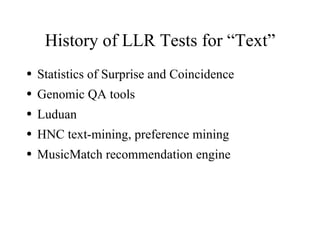
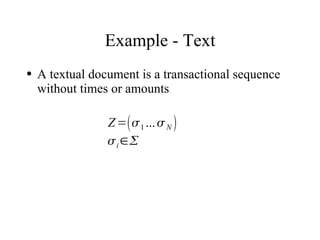
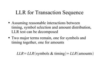
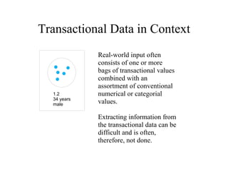
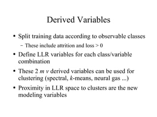
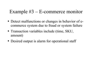
17. Transaction Sequence Distributions
● Mixed Poisson distributions give desired
symbol/timing behavior
● Amount distribution depends on symbol
k  − T
 T  e
pZ = ∏ ∏ p x i∣  
 ∈ k ! i=1. .. N
i
[ ][ ]∏
k − T
 N
T  e
pZ = N ! ∏

p x i∣  
∈ k  ! N! i
i=1. .. N
 = , ∑  =1
 ∈

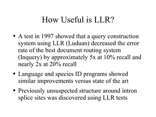
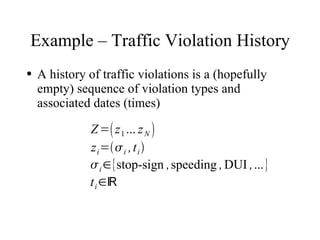
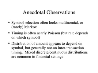
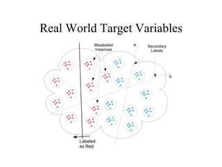
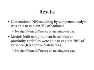
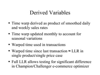
18. LLR for Multinomial
● Easily expressed as entropy of contingency table
[ ]
k 11 k 12 ... k1 n k 1*
k 21 k 22 ... k2n k 2*
⋮ ⋮ ⋱ ⋮ ⋮
k m1 k m2 ... k mn k m*
k * 1 k * 2 ... k * n k **
−2 log =2 N
 ∑ ij log ij −∑ i * log i *−∑ * j log * j 
ij i j
k ij k ** ij
log =∑ k ij log =∑ k ij log d.o.f.=m−1n−1
ij k i * k * j ij * j

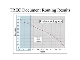
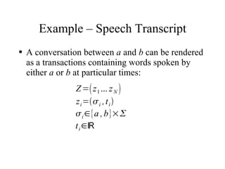
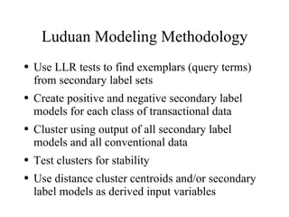
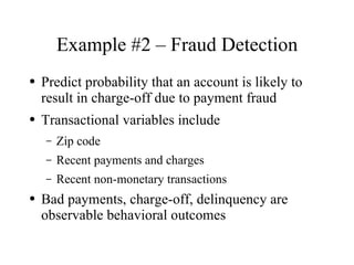
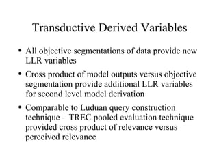
19. LLR for Poisson Mixture
● Easily expressed using timed contingency table
[ ∣]
k 11 k 12 ... k1n t1
k 21 k 22 ... k 2n t2
⋮ ⋮ ⋱ ⋮ ⋮
k m1 k m2 ... k mn tm
k * 1 k * 2 ... k * n ∣ t *
k ij t * ij
log =∑ k ij log =∑ k ij log
ij t i k * j ij * j
d.o.f.=m−1 n

20. LLR for Normal Distribution
● Assume X1 and X2 are normally distributed
● Null hypothesis of identical mean and variance

− x−2
p  x∣ ,  =
1
e 2 2

=
∑ xi 
=
∑  x i −2
 2  N N


−2 log =2 N 1 log N 2 log

1



2 
d.o.f.=2

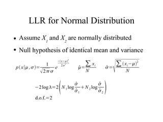
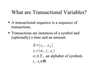
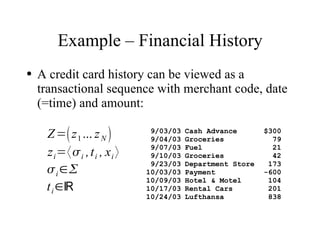
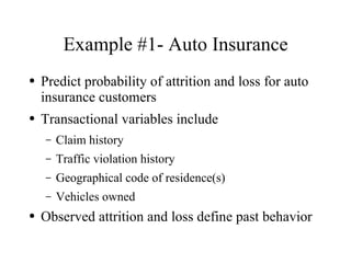
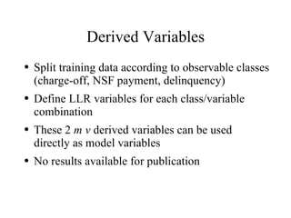
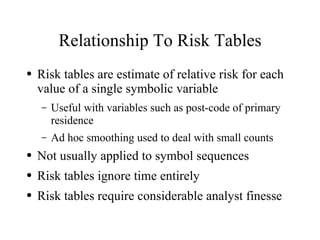
21. Calculations
● Assume X1 and X2 are normally distributed
● Null hypothesis of identical mean and variance
p  x∣ ,=
1
 2 
e
− x−2
2 2
= i

N
∑ xi
= i

N
∑  x−2
log p X 1∣ ,  log p X 1∣ , −log p X 1∣1,  1 −log p X 2∣2,  2 =
− ∑ [
i=1. . N 1
log  2 log 
 x 1i −2
2 2 ] [
− ∑ log  2 log 
i=1. . N
2
 x 2 i −2
2 2 ]
∑ [ ] ∑[ ]
2 2
 x −   x − 
 log  2 log  1  1i 2 1  log  2 log  2 2i 2 2
i=1. . N 1 2 1 i=1. . N 2
2 2
−2 log =2 N 1 log
 
1
N 2 log

2 
d.o.f.=2

22. Transactional Data in Context
Real-world input often
consists of one or more
bags of transactional values
combined with an
assortment of conventional
1.2 numerical or categorial
34 years
male values.
Extracting information from
the transactional data can be
difficult and is often,
therefore, not done.

23. Real World Target Variables
Mislabeled a Secondary
Instances Labels
b
Labeled
as Red

24. Luduan Modeling Methodology
● Use LLR tests to find exemplars (query terms)
from secondary label sets
● Create positive and negative secondary label
models for each class of transactional data
● Cluster using output of all secondary label
models and all conventional data
● Test clusters for stability
● Use distance cluster centroids and/or secondary
label models as derived input variables

25. Example #1- Auto Insurance
● Predict probability of attrition and loss for auto
insurance customers
● Transactional variables include
– Claim history
– Traffic violation history
– Geographical code of residence(s)
– Vehicles owned
● Observed attrition and loss define past behavior

26. Derived Variables
● Split training data according to observable classes
– These include attrition and loss > 0
● Define LLR variables for each class/variable
combination
● These 2 m v derived variables can be used for
clustering (spectral, k-means, neural gas ...)
● Proximity in LLR space to clusters are the new
modeling variables

27. Results
● Conventional NN modeling by competent analyst
was able to explain 2% of variance
– No significant difference on training/test data
● Models built using Luduan based cluster
proximity variables were able to explain 70% of
variance (KS approximately 0.4)
– No significant difference on training/test data

28. Example #2 – Fraud Detection
● Predict probability that an account is likely to
result in charge-off due to payment fraud
● Transactional variables include
– Zip code
– Recent payments and charges
– Recent non-monetary transactions
● Bad payments, charge-off, delinquency are
observable behavioral outcomes

29. Derived Variables
● Split training data according to observable classes
(charge-off, NSF payment, delinquency)
● Define LLR variables for each class/variable
combination
● These 2 m v derived variables can be used
directly as model variables
● No results available for publication

30. Example #3 – E-commerce monitor
● Detect malfunctions or changes in behavior of e-
commerce system due to fraud or system failure
● Transaction variables include (time, SKU,
amount)
● Desired output is alarm for operational staff

31. Derived Variables
● Time warp derived as product of smoothed daily
and weekly sales rates
● Time warp updated monthly to account for
seasonal variations
● Warped time used in transactions
● Warped time since last transaction ≈ LLR in
single product/single price case
● Full LLR allows testing for significant difference
in Champion/Challenger e-commerce optimizer

32. Transductive Derived Variables
● All objective segmentations of data provide new
LLR variables
● Cross product of model outputs versus objective
segmentation provide additional LLR variables
for second level model derivation
● Comparable to Luduan query construction
technique – TREC pooled evaluation technique
provided cross product of relevance versus
perceived relevance

33. Relationship To Risk Tables
● Risk tables are estimate of relative risk for each
value of a single symbolic variable
– Useful with variables such as post-code of primary
residence
– Ad hoc smoothing used to deal with small counts
● Not usually applied to symbol sequences
● Risk tables ignore time entirely
● Risk tables require considerable analyst finesse

34. Relationship to Known Techniques
● Clock-tick symbols
– Time-embedded symbols viewed as sequences of
symbols along with “ticks” that occur at fixed time
intervals
– Allows multinomial LLR as poor man's mixed
Poisson LLR
● Not a well known technique, not used in
production models
● Difficulties in choosing time resolution and
counting period

35. Conclusions
● Theoretical properties of transaction variables are
well defined
● Similarities to known techniques indicates low
probability of gross failure
● Similarity to Luduan techniques suggests high
probability of superlative performance
● Transactional LLR statistics define similarity
metrics useful for clustering