The document discusses challenges and solutions in approximate data computation, focusing on speed, feasibility, and communication issues. It highlights classic problems such as finding the most common elements, counting distinct elements, and calculating quantiles, presenting techniques like leaky counters, count min sketch, and hyperloglog for effective solutions. Additionally, it introduces a new method using t-digest for improved quantile accuracy, particularly at extremes.


![© 2014 MapR Technologies 11
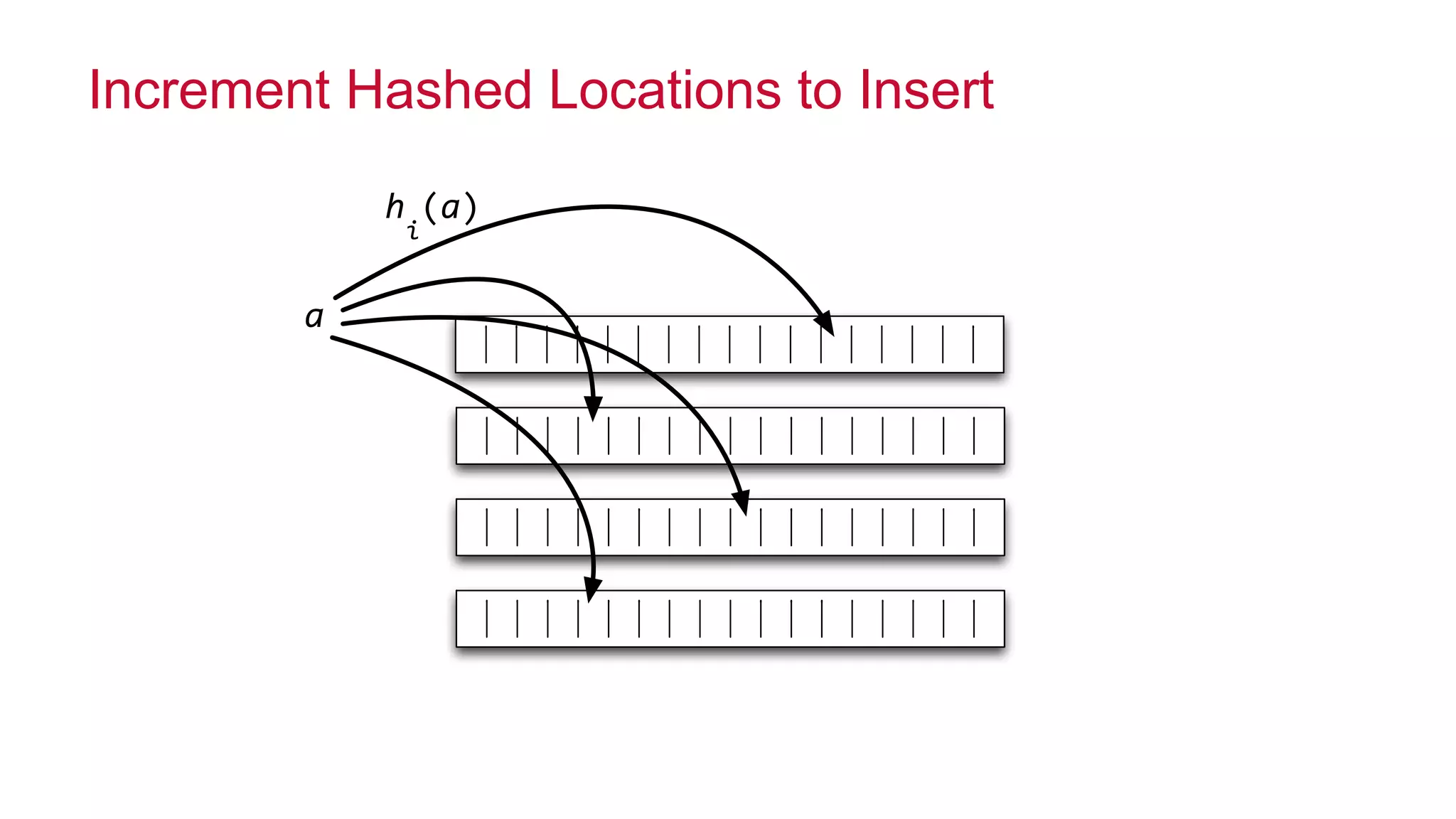
Probe Using min of Counts
mini"k[h
i
(a)]](https://image.slidesharecdn.com/strata-2014-doing-the-impossible-141020022735-conversion-gate02/75/Doing-the-impossible-11-2048.jpg)


![Vibe Coding vs. Spec-Driven Development [Free Meetup]](https://cdn.slidesharecdn.com/ss_thumbnails/vibecodingvsspecdrivendevelopment-251209105622-43f455e7-thumbnail.jpg?width=640&height=640&fit=bounds)


