This document discusses dynamic programming and greedy algorithms. It begins by defining dynamic programming as a technique for solving problems with overlapping subproblems. It provides examples of dynamic programming approaches to computing Fibonacci numbers, binomial coefficients, the knapsack problem, and other problems. It also discusses greedy algorithms and provides examples of their application to problems like the change-making problem, minimum spanning trees, and single-source shortest paths.

1. Unit 3
DYNAMIC PROGRAMMING
AND GREEDY APPROACH
Dr.S.Gunasundari
Associate Professor
CSE Dept

2. Dynamic Programming
Dynamic Programming is a general algorithm design technique
for solving problems defined by recurrences with overlapping
subproblems
• Invented by American mathematician Richard Bellman in the
1950s to solve optimization problems and later assimilated by CS
• “Programming” here means “planning”
• Main idea:
- set up a recurrence relating a solution to a larger instance
to solutions of some smaller instances
- solve smaller instances once
- record solutions in a table
- extract solution to the initial instance from that table

3. Example: Fibonacci numbers
• Recall definition of Fibonacci numbers:
F(n) = F(n-1) + F(n-2)
F(0) = 0
F(1) = 1
• Computing the nth Fibonacci number recursively (top-down):
F(n)
F(n-1) + F(n-2)
F(n-2) + F(n-3) F(n-3) + F(n-4)
...

4. Example: Fibonacci numbers (cont.)
Computing the nth Fibonacci number using bottom-up iteration and
recording results:
F(0) = 0
F(1) = 1
F(2) = 1+0 = 1
…
F(n-2) =
F(n-1) =
F(n) = F(n-1) + F(n-2)
Efficiency:
- time
- space
0 1 1 . . . F(n-2) F(n-1) F(n)

5. Examples of DP algorithms
• Computing a binomial coefficient
• Warshall’s algorithm for transitive closure
• Floyd’s algorithm for all-pairs shortest paths
• Constructing an optimal binary search tree
• Some instances of difficult discrete optimization problems:
- traveling salesman
- knapsack

6. Computing a binomial coefficient by DP
Binomial coefficients are coefficients of the binomial formula:
(a + b)n = C(n,0)anb0 + . . . + C(n,k)an-kbk + . . . + C(n,n)a0bn
Recurrence: C(n,k) = C(n-1,k) + C(n-1,k-1) for n > k > 0
C(n,0) = 1, C(n,n) = 1 for n  0
Value of C(n,k) can be computed by filling a table:
0 1 2 . . . k-1 k
0 1
1 1 1
.
.
.
n-1 C(n-1,k-1) C(n-1,k)
n C(n,k)

7. Computing C(n,k): pseudocode and
analysis
Time efficiency: Θ(nk)
Space efficiency: Θ(nk)

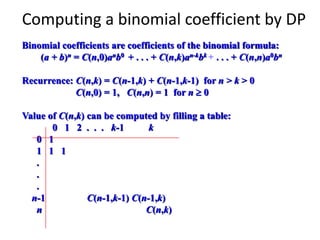
8. Knapsack Problem by DP
Given n items of
integer weights: w1 w2 … wn
values: v1 v2 … vn
a knapsack of integer capacity W
find most valuable subset of the items that fit into the
knapsack
Consider instance defined by first i items and capacity
j (j  W).
Let V[i,j] be optimal value of such instance. Then
max {V[i-1,j], vi + V[i-1,j- wi]} if j- wi  0
V[i,j] =
V[i-1,j] if j- wi < 0
Initial conditions: V[0,j] = 0 and V[i,0] = 0

9. Knapsack Problem by DP (example)
Example: Knapsack of capacity W = 5
item weight value
1 2 $12
2 1 $10
3 3 $20
4 2 $15 capacity j
0 1 2 3 4 5
0
w1 = 2, v1= 12 1
w2 = 1, v2= 10 2
w3 = 3, v3= 20 3
w4 = 2, v4=15 4 ?

10. Warshall’s Algorithm: Transitive Closure
• Computes the transitive closure of a relation
• Alternatively: existence of all nontrivial paths in a digraph
• Example of transitive closure:
3
4
2
1
0 0 1 0
1 0 0 1
0 0 0 0
0 1 0 0
0 0 1 0
1 1 1 1
0 0 0 0
1 1 1 1
3
4
2
1

11. Warshall’s Algorithm
Constructs transitive closure T as the last matrix in the sequence
of n-by-n matrices R(0), … , R(k), … , R(n) where
R(k)[i,j] = 1 iff there is nontrivial path from i to j with only first k
vertices allowed as intermediate
Note that R(0) = A (adjacency matrix), R(n) = T (transitive closure)
3
4
2
1
3
4
2
1
3
4
2
1
3
4
2
1
R(0)
0 0 1 0
1 0 0 1
0 0 0 0
0 1 0 0
R(1)
0 0 1 0
1 0 1 1
0 0 0 0
0 1 0 0
R(2)
0 0 1 0
1 0 1 1
0 0 0 0
1 1 1 1
R(3)
0 0 1 0
1 0 1 1
0 0 0 0
1 1 1 1
R(4)
0 0 1 0
1 1 1 1
0 0 0 0
1 1 1 1
3
4
2
1

12. Warshall’s Algorithm (recurrence)
On the k-th iteration, the algorithm determines for every pair of vertices i, j if a path
exists from i and j with just vertices 1,…,k allowed as intermediate
R(k-1)[i,j] (path using just 1 ,…,k-1)
R(k)[i,j] = or
R(k-1)[i,k] and R(k-1)[k,j] (path from i to k
and from k to i
using just 1 ,…,k-1)
i
j
k
{

13. Warshall’s Algorithm (matrix generation)
Recurrence relating elements R(k) to elements of R(k-1) is:
R(k)[i,j] = R(k-1)[i,j] or (R(k-1)[i,k] and R(k-1)[k,j])
It implies the following rules for generating R(k) from R(k-1):
Rule 1 If an element in row i and column j is 1 in R(k-1),
it remains 1 in R(k)
Rule 2 If an element in row i and column j is 0 in R(k-1),
it has to be changed to 1 in R(k) if and only if
the element in its row i and column k and the element
in its column j and row k are both 1’s in R(k-1)

14. Warshall’s Algorithm (example)
3
4
2
1
0 0 1 0
1 0 0 1
0 0 0 0
0 1 0 0
R(0) =
0 0 1 0
1 0 1 1
0 0 0 0
0 1 0 0
R(1) =
0 0 1 0
1 0 1 1
0 0 0 0
1 1 1 1
R(2) =
0 0 1 0
1 0 1 1
0 0 0 0
1 1 1 1
R(3) =
0 0 1 0
1 1 1 1
0 0 0 0
1 1 1 1
R(4) =

15. Warshall’s Algorithm (pseudocode and analysis)
Time efficiency: Θ(n3)
Space efficiency: Matrices can be written over their predecessors

16. Floyd’s Algorithm: All pairs shortest paths
Problem: In a weighted (di)graph, find shortest paths between
every pair of vertices
Same idea: construct solution through series of matrices D(0), …,
D (n) using increasing subsets of the vertices allowed
as intermediate
Example:
3
4
2
1
4
1
6
1
5
3

17. Floyd’s Algorithm (matrix generation)
On the k-th iteration, the algorithm determines shortest paths
between every pair of vertices i, j that use only vertices among
1,…,k as intermediate
D(k)[i,j] = min {D(k-1)[i,j], D(k-1)[i,k] + D(k-1)[k,j]}
i
j
k
D(k-1)[i,j]
D(k-1)[i,k]
D(k-1)[k,j]

18. Floyd’s Algorithm (example)
0 ∞ 3 ∞ 2
0 ∞ ∞
∞ 7 0 1
6 ∞ ∞ 0
D(0) =
0 ∞ 3 ∞
2 0 5 ∞
∞ 7 0 1
6 ∞ 9 0
D(1) =
0 ∞ 3 ∞
2 0 5 ∞
9 7 0 1
6 ∞ 9 0
D(2) =
0 10 3 4
2 0 5 6
9 7 0 1
6 16 9 0
D(3) =
0 10 3 4
2 0 5 6
7 7 0 1
6 16 9 0
D(4) =
3 1
3
2
6 7
4
1 2

19. Floyd’s Algorithm (pseudocode and analysis)
Time efficiency: Θ(n3)
Space efficiency: Matrices can be written over their predecessors
Note: Shortest paths themselves can be found, too

20. Optimal Binary Search Trees
Problem: Given n keys a1 < …< an and probabilities p1 ≤ … ≤ pn
searching for them, find a BST with a minimum
average number of comparisons in successful search.
Since total number of BSTs with n nodes is given by C(2n,n)/(n+1), which grows
exponentially, brute force is hopeless.
Example: What is an optimal BST for keys A, B, C, and D with
search probabilities 0.1, 0.2, 0.4, and 0.3, respectively?

21. DP for Optimal BST Problem
a
Optimal
BST for
a , ..., a
Optimal
BST for
a , ..., a
i
k
k-1 k+1 j
Let C[i,j] be minimum average number of comparisons made in T[i,j], optimal BST for keys
ai < …< aj , where 1 ≤ i ≤ j ≤ n. Consider optimal BST among all BSTs with some ak (i ≤ k ≤
j ) as their root; T[i,j] is the best among them.
C[i,j] =
min {pk · 1 +
∑ ps (level as in T[i,k-1] +1) +
∑ ps (level as in T[k+1,j] +1)}
i ≤ k ≤ j
s = i
k-1
s =k+1
j

22. DP for Optimal BST Problem (cont.)
After simplifications, we obtain the recurrence for C[i,j]:
C[i,j] = min {C[i,k-1] + C[k+1,j]} + ∑ ps for 1 ≤ i ≤ j ≤ n
C[i,i] = pi for 1 ≤ i ≤ j ≤ n
s = i
j
i ≤ k ≤ j

23. Example: key A B C D
probability 0.1 0.2 0.4 0.3
The tables below are filled diagonal by diagonal: the left one is filled using the recurrence
C[i,j] = min {C[i,k-1] + C[k+1,j]} + ∑ ps , C[i,i] = pi ;
the right one, for trees’ roots, records k’s values giving the minima
0 1 2 3 4
1 0 .1 .4 1.1 1.7
2 0 .2 .8 1.4
3 0 .4 1.0
4 0 .3
5 0
0 1 2 3 4
1 1 2 3 3
2 2 3 3
3 3 3
4 4
5
i ≤ k ≤ j s = i
j
optimal BST
B
A
C
D
i
j
i
j

24. Optimal Binary Search Trees

25. Analysis DP for Optimal BST Problem
Time efficiency: Θ(n3) but can be reduced to Θ(n2) by taking
advantage of monotonicity of entries in the
root table, i.e., R[i,j] is always in the range
between R[i,j-1] and R[i+1,j]
Space efficiency: Θ(n2)
Method can be expended to include unsuccessful searches

26. Greedy Technique
Constructs a solution to an optimization problem piece by
piece through a sequence of choices that are:
• feasible
• locally optimal
• irrevocable
For some problems, yields an optimal solution for every
instance.
For most, does not but can be useful for fast approximations.

27. Applications of the Greedy Strategy
• Optimal solutions:
– change making for “normal” coin denominations
– minimum spanning tree (MST)
– single-source shortest paths
– simple scheduling problems
– Huffman codes
• Approximations:
– traveling salesman problem (TSP)
– knapsack problem
– other combinatorial optimization problems

28. Change-Making Problem
Given unlimited amounts of coins of denominations d1 > … >
dm ,
give change for amount n with the least number of coins
Example: d1 = 25c, d2 =10c, d3 = 5c, d4 = 1c and n = 48c
Greedy solution:
Greedy solution is
• optimal for any amount and “normal’’ set of
denominations
• may not be optimal for arbitrary coin denominations

29. Minimum Spanning Tree (MST)
• Spanning tree of a connected graph G: a
connected acyclic subgraph of G that includes
all of G’s vertices
• Minimum spanning tree of a weighted,
connected graph G: a spanning tree of G of
minimum total weight
Example:
c
d
b
a
6
2
4
3
1

30. Prim’s MST algorithm
• Start with tree T1 consisting of one (any) vertex
and “grow” tree one vertex at a time to
produce MST through a series of expanding
subtrees T1, T2, …, Tn
• On each iteration, construct Ti+1 from Ti by
adding vertex not in Ti that is closest to those
already in Ti (this is a “greedy” step!)
• Stop when all vertices are included

31. Example
c
d
b
a
4
2
6
1
3

32. Notes about Prim’s algorithm
• Proof by induction that this construction actually
yields MST
• Needs priority queue for locating closest fringe
vertex
• Efficiency
– O(n2) for weight matrix representation of graph and array
implementation of priority queue
– O(m log n) for adjacency list representation of graph with n
vertices and m edges and min-heap implementation of priority
queue

33. Another greedy algorithm for MST: Kruskal’s
• Sort the edges in nondecreasing order of lengths
• “Grow” tree one edge at a time to produce MST
through a series of expanding forests F1, F2, …, Fn-
1
• On each iteration, add the next edge on the
sorted list unless this would create a cycle. (If it
would, skip the edge.)

34. Example
c
d
b
a
4
2
6
1
3

35. Notes about Kruskal’s algorithm
• Algorithm looks easier than Prim’s but is
harder to implement (checking for cycles!)
• Cycle checking: a cycle is created iff added
edge connects vertices in the same connected
component
• Union-find algorithms – see section 9.2

36. Shortest paths – Dijkstra’s algorithm
Single Source Shortest Paths Problem: Given a weighted
connected graph G, find shortest paths from source vertex s
to each of the other vertices
Dijkstra’s algorithm: Similar to Prim’s MST algorithm, with
a different way of computing numerical labels: Among vertices
not already in the tree, it finds vertex u with the smallest sum
dv + w(v,u)
where
v is a vertex for which shortest path has been already found
on preceding iterations (such vertices form a tree)
dv is the length of the shortest path form source to v
w(v,u) is the length (weight) of edge from v to u

37. d
4
Tree vertices Remaining vertices
a(-,0) b(a,3) c(-,∞) d(a,7) e(-,∞)
a
b
4
e
3
7
6
2 5
c
a
b
d
4
c
e
3
7 4
6
2 5
a
b
d
4
c
e
3
7 4
6
2 5
a
b
d
4
c
e
3
7 4
6
2 5
b(a,3) c(b,3+4) d(b,3+2) e(-,∞)
d(b,5) c(b,7) e(d,5+4)
c(b,7) e(d,9)
e(d,9)
d
a
b
d
4
c
e
3
7 4
6
2 5

38. Notes on Dijkstra’s algorithm
• Doesn’t work for graphs with negative weights
• Applicable to both undirected and directed graphs
• Efficiency
– O(|V|2) for graphs represented by weight matrix and array
implementation of priority queue
– O(|E|log|V|) for graphs represented by adj. lists and min-heap
implementation of priority queue
• Don’t mix up Dijkstra’s algorithm with Prim’s algorithm!

39. Coding Problem
Coding: assignment of bit strings to alphabet characters
Codewords: bit strings assigned for characters of alphabet
Two types of codes:
• fixed-length encoding (e.g., ASCII)
• variable-length encoding (e,g., Morse code)
Prefix-free codes: no codeword is a prefix of another codeword
Problem: If frequencies of the character occurrences are
known, what is the best binary prefix-free code?

40. Huffman codes
• Any binary tree with edges labeled with 0’s and 1’s yields a prefix-free code of
characters assigned to its leaves
• Optimal binary tree minimizing the expected (weighted average) length of a
codeword can be constructed as follows
Huffman’s algorithm
Initialize n one-node trees with alphabet characters and the tree weights with
their frequencies.
Repeat the following step n-1 times: join two binary trees with smallest weights
into one (as left and right subtrees) and make its weight equal the sum of the
weights of the two trees.
Mark edges leading to left and right subtrees with 0’s and 1’s, respectively.

41. Example
character A B C D _
frequency 0.35 0.1 0.2 0.2 0.15
codeword 11 100 00 01 101
average bits per character: 2.25
for fixed-length encoding: 3
compression ratio: (3-2.25)/3*100% = 25%
0.25
0.1
B
0.15
_
0.2
C
0.2
D
0.35
A
0.2
C
0.2
D
0.35
A
0.1
B
0.15
_
0.4
0.2
C
0.2
D
0.6
0.25
0.1
B
0.15
_
0.6
1.0
0 1
0.4
0.2
C
0.2
D
0.25
0.1
B
0.15
_
0 1 0
0
1
1
0.25
0.1
B
0.15
_
0.35
A
0.4
0.2
C
0.2
D
0.35
A
0.35
A