Downloaded 148 times
![Partitioning
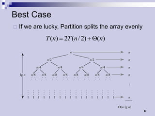
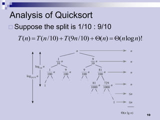
Linear time partitioning procedure
Partition(A,p,r) i i j j
01 x A[r] 17 12 6 19 23 8 5 10
02 i p-1
03 j r+1 X=10 i j
04 while TRUE
10 12 6 19 23 8 5 17
05 repeat j j-1
06 until A[j] x
i j
07 repeat i i+1
08 until A[i] x 10 5 6 19 23 8 12 17
09 if i<j
10 then exchange A[i] A[j]
j i
11 else return j
10 5 6 8 23 19 12 17
3](https://image.slidesharecdn.com/lec10-101217101413-phpapp02/85/Lec10-3-320.jpg)
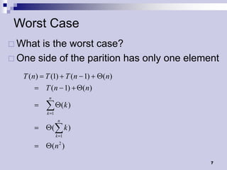
![Quick Sort Algorithm
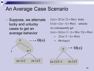
Initial call Quicksort(A, 1, length[A])
Quicksort(A,p,r)
01 if p<r
02 then q Partition(A,p,r)
03 Quicksort(A,p,q)
04 Quicksort(A,q+1,r)
4](https://image.slidesharecdn.com/lec10-101217101413-phpapp02/85/Lec10-4-320.jpg)
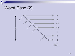
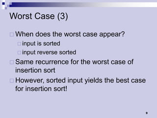
![Randomized Quicksort (2)
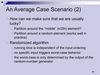
Randomized-Partition(A,p,r)
01 i Random(p,r)
02 exchange A[r] A[i]
03 return Partition(A,p,r)
Randomized-Quicksort(A,p,r)
01 if p < r then
02 q Randomized-Partition(A,p,r)
03 Randomized-Quicksort(A,p,q)
04 Randomized-Quicksort(A,q+1,r)
14](https://image.slidesharecdn.com/lec10-101217101413-phpapp02/85/Lec10-14-320.jpg)
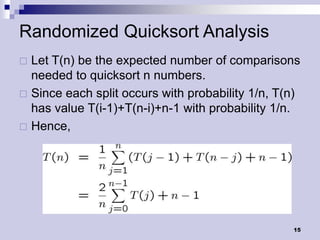

Quicksort is a divide-and-conquer algorithm that works by partitioning an array into two subarrays such that elements in one subarray are less than the elements in the other. It then recursively sorts the subarrays. The average runtime is O(n log n) but the worst case is O(n^2) when the array is already sorted. Randomizing the pivot selection results in an expected runtime of O(n log n) for all cases.