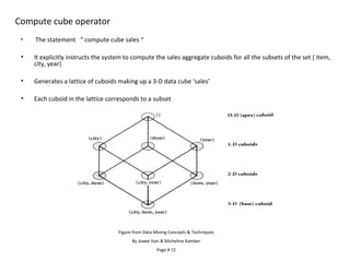
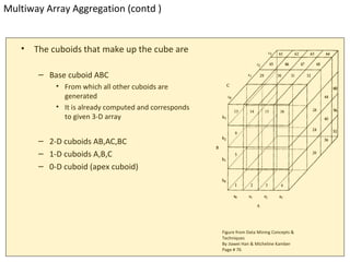
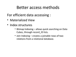
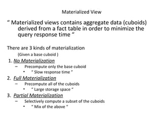
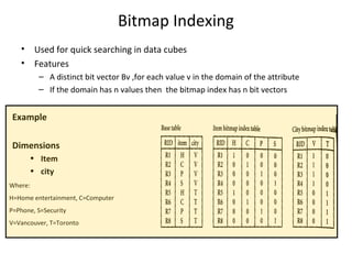
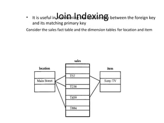
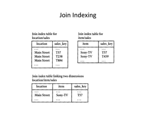
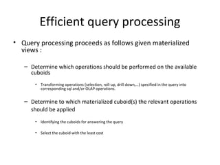
The document discusses data warehouse implementation and online analytical processing (OLAP). It describes the compute cube operator, which computes aggregates for all subsets of specified dimensions. It also covers efficient cube computation techniques like chunking and materialized views. Better access methods for OLAP like bitmap indexing and join indexing are also summarized. The document emphasizes that efficient query processing requires determining which operations to perform on available cuboids and selecting the optimal cuboid based on factors like storage size and indexing.

1. Data warehouse implementation

2. “ What is the Challenge ? “
– Faster processing of OLAP queries
Requirements of a Data Warehouse system
 Efficient cube computation
 Better access methods
 Efficient query processing

3. Cube computation
COMPUTE CUBE OPERATOR
 Definition :
“ It computes the aggregates over all subsets of the
dimensions specified in the operation “
Syntax :
Compute cube cubename
Example
Consider we define the data cube for an electronic store “Best Electronics”
Dimensions are :
City
Item
Year
Measure :
Sales_in_dollars

4. Cube Operation
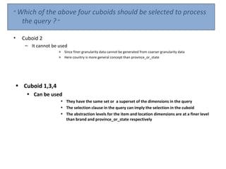
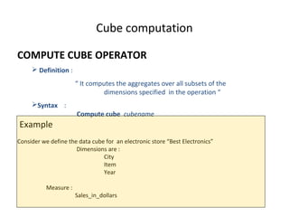
• Cube definition and computation in DMQL
define cube sales[item, city, year]: sum(sales_in_dollars)
compute cube sales
• Transform it into a SQL-like language (with a new operator cube by,
introduced by Gray et al.’96) ()
SELECT item, city, year, SUM (amount)
FROM SALES (city) (item) (year)
CUBE BY item, city, year
• Need compute the following Group-Bys
(city, item) (city, year) (item, year)
(date, product, customer),
(date,product),(date, customer), (product, customer),
(date), (product), (customer) (city, item, year)
() 4

5. Efficient Data Cube Computation
• Data cube can be viewed as a lattice of cuboids
– The bottom-most cuboid is the base cuboid
– The top-most cuboid (apex) contains only one cell
– How many cuboids in an n-dimensional cube with L levels?
n
T = ∏ ( Li + )
1
i= 1
• Materialization of data cube
– Materialize every (cuboid) (full materialization), none (no
materialization), or some (partial materialization)
– Selection of which cuboids to materialize
• Based on size, sharing, access frequency, etc.
5

6. Iceberg Cube
• Computing only the cuboid cells whose count
or other aggregates satisfying the condition like
HAVING COUNT(*) >= minsup
 Motivation
 Only a small portion of cube cells may be “above the water’’
in a sparse cube
 Only calculate “interesting” cells—data above certain
threshold
 Avoid explosive growth of the cube
Suppose 100 dimensions, only 1 base cell. How many aggregate cells if
6

7. Compute cube operator
• The statement “ compute cube sales “
• It explicitly instructs the system to compute the sales aggregate cuboids for all the subsets of the set { item,
city, year}
• Generates a lattice of cuboids making up a 3-D data cube ‘sales’
• Each cuboid in the lattice corresponds to a subset
Figure from Data Mining Concepts & Techniques
By Jiawei Han & Micheline Kamber
Page # 72

8. Compute cube operator
 Advantages
– Computes all the cuboids for the cube in advance
– Online analytical processing needs to access different cuboids for different queries.
– Precomputation leads to fast response time
 Disadvantages
– Required storage space may explode if all of the cuboids in the data cube are
precomputed
• Consider the following 2 cases for n-dimensional cube
– Case 1 : Dimensions have no hierarchies
• Then the total number of cuboids computed for a n-dimensional cube = 2n
– Case 2: Dimensions have hierarchies
• Then the total number of cuboids computed for a n-dimensional cube =
» Where Li is the number of levels associated with dimension i

9. Multiway Array Aggregation
“ What is chunking ?”
• MOLAP uses multidimensional array for data storage
• Chunk is obtained by partitioning the multidimensional array such that it
is small enough to fit in the memory available for cube computation
So from the above 2 points we get :
“ Chunking is a method for dividing the n-dimensional array into small n-
dimensional chunks “

10. Multiway Array Aggregation
• It is a technique used for the computation of data cube
• It is used for MOLAP cube construction
Example
• Consider 3-D data array
• Dimensions are A,B,C
• Each dimension is partitioned into 4
equalized partitions
• A : a0,a1,a2,a3
• B : b0,b1,b2,b3
• C : c0,c1,c2,c3
• 3-D array is partitioned into 64 chunks as
shown in the figure
Figure from Data Mining Concepts & Techniques
By Jiawei Han & Micheline Kamber
Page # 76

11. Multiway Array Aggregation (contd )
• The cuboids that make up the cube are
– Base cuboid ABC
• From which all other cuboids are
generated
• It is already computed and corresponds
to given 3-D array
– 2-D cuboids AB,AC,BC
– 1-D cuboids A,B,C
– 0-D cuboid (apex cuboid)
Figure from Data Mining Concepts &
Techniques
By Jiawei Han & Micheline Kamber
Page # 76

12. Better access methods
For efficient data accessing :
• Materialized View
• Index structures
• Bitmap Indexing – allows quick searching on Data
Cubes, through record_ID lists.
• Join Indexing – creates a joinable rows of two
relations from a relational database.

13. Materialized View
“ Materialized views contains aggregate data (cuboids)
derived from a fact table in order to minimize the
query response time “
There are 3 kinds of materialization
(Given a base cuboid )
1. No Materialization
– Precompute only the base cuboid
• “ Slow response time ”
2. Full Materialization
– Precompute all of the cuboids
• “ Large storage space “
3. Partial Materialization
– Selectively compute a subset of the cuboids
• “ Mix of the above “

14. Bitmap Indexing
• Used for quick searching in data cubes
• Features
– A distinct bit vector Bv ,for each value v in the domain of the attribute
– If the domain has n values then the bitmap index has n bit vectors
Example
Dimensions
• Item
• city
Where:
H=Home entertainment, C=Computer
P=Phone, S=Security
V=Vancouver, T=Toronto

15. Join Indexing
• It is useful in maintaining the relationship between the foreign key
and its matching primary key
Consider the sales fact table and the dimension tables for location and item

16. Join Indexing

17. Efficient query processing
• Query processing proceeds as follows given materialized
views :
– Determine which operations should be performed on the available
cuboids
• Transforming operations (selection, roll-up, drill down,…) specified in the query into
corresponding sql and/or OLAP operations.
– Determine to which materialized cuboid(s) the relevant operations
should be applied
• Identifying the cuboids for answering the query
• Select the cuboid with the least cost

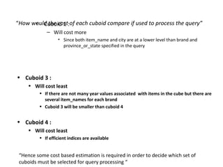
18. Consider a data cube for “Best Electronics” of the form
• “sales [time, item, location]:sum(sales_in_dollars)
• Dimension hierarchies used are :
– “ day<month<quarter<year ” for time
– “ item_name<brand<type” for item
– “ street<city<province_or_state<country “ for location
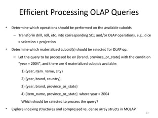
• Query :{ brand,province_or_state} with year = 2000
• Materialized cuboids available are
• Cuboid 1: { item_name,city,year}
• Cuboid 2: {brand,country,year}
• Cuboid 3: {brand,province_or_state,year}
• Cuboid 4: {item_name,province_or_state} where year=2000

19. “ Which of the above four cuboids should be selected to process
the query ? “
• Cuboid 2
– It cannot be used
» Since finer granularity data cannot be generated from coarser granularity data
» Here country is more general concept than province_or_state
• Cuboid 1,3,4
• Can be used
• They have the same set or a superset of the dimensions in the query
• The selection clause in the query can imply the selection in the cuboid
• The abstraction levels for the item and location dimensions are at a finer level
than brand and province_or_state respectively

20. “How would the cost:of each cuboid compare if used to process the query”
• Cuboid 1
– Will cost more
• Since both item_name and city are at a lower level than brand and
province_or_state specified in the query
• Cuboid 3 :
• Will cost least
• If there are not many year values associated with items in the cube but there are
several item_names for each brand
• Cuboid 3 will be smaller than cuboid 4
• Cuboid 4 :
• Will cost least
• If efficient indices are available
“Hence some cost based estimation is required in order to decide which set of
cuboids must be selected for query processing “

21. Indexing OLAP Data: Bitmap Index
• Index on a particular column
• Each value in the column has a bit vector: bit-op is fast
• The length of the bit vector: # of records in the base table
• The i-th bit is set if the i-th row of the base table has the value for the
indexed column
• not suitable for high cardinality domains
Base table Index on Region Index on Type
Cust Region Type RecIDAsia Europe America RecID Retail Dealer
C1 Asia Retail 1 1 0 0 1 1 0
C2 Europe Dealer 2 0 1 0 2 0 1
C3 Asia Dealer 3 1 0 0 3 0 1
C4 America Retail 4 0 0 1 4 1 0
C5 Europe Dealer 5 0 1 0 5 0 1
21

22. Indexing OLAP Data: Join Indices
• Join index: JI(R-id, S-id) where R (R-id, …)  S (S-id,
…)
• Traditional indices map the values to a list of record
ids
– It materializes relational join in JI file and speeds
up relational join
• In data warehouses, join index relates the values of
the dimensions of a start schema to rows in the fact
table.
– E.g. fact table: Sales and two dimensions city and
product
• A join index on city maintains for each distinct
city a list of R-IDs of the tuples recording the
Sales in the city
– Join indices can span multiple dimensions
22

23. Efficient Processing OLAP Queries
• Determine which operations should be performed on the available cuboids
– Transform drill, roll, etc. into corresponding SQL and/or OLAP operations, e.g., dice
= selection + projection
• Determine which materialized cuboid(s) should be selected for OLAP op.
– Let the query to be processed be on {brand, province_or_state} with the condition
“year = 2004”, and there are 4 materialized cuboids available:
1) {year, item_name, city}
2) {year, brand, country}
3) {year, brand, province_or_state}
4) {item_name, province_or_state} where year = 2004
Which should be selected to process the query?
• Explore indexing structures and compressed vs. dense array structs in MOLAP
23

24. From data warehousing to data mining
24

25. Data Warehouse Usage
• Three kinds of data warehouse applications
– Information processing
• supports querying, basic statistical analysis, and reporting using
crosstabs, tables, charts and graphs
– Analytical processing
• multidimensional analysis of data warehouse data
• supports basic OLAP operations, slice-dice, drilling, pivoting
– Data mining
• knowledge discovery from hidden patterns
• supports associations, constructing analytical models, performing
classification and prediction, and presenting the mining results
using visualization tools
25

26. From On-Line Analytical Processing (OLAP)
to On Line Analytical Mining (OLAM)
• Why online analytical mining?
– High quality of data in data warehouses
• DW contains integrated, consistent, cleaned data
– Available information processing structure surrounding data
warehouses
• ODBC, OLEDB, Web accessing, service facilities, reporting
and OLAP tools
– OLAP-based exploratory data analysis
• Mining with drilling, dicing, pivoting, etc.
– On-line selection of data mining functions
• Integration and swapping of multiple mining functions,
algorithms, and tasks
26

27. An OLAM System Architecture
Mining query Mining result Layer4
User Interface
User GUI API
Layer3
OLAM OLAP
Engine Engine OLAP/OLAM
Data Cube API
Layer2
MDDB
MDDB
Meta
Data
Filtering&Integration Database API Filtering
Layer1
Data cleaning Data
Databases Data
Data integration Warehouse Repository
27

28. OLAP APPLICATIONS
• Financial Applications
• Activity-based costing (resource allocation)
• Budgeting
• Marketing/Sales Applications
• Market Research Analysis
• Sales Forecasting
• Promotions Analysis
• Customer Analyses
• Market/Customer Segmentation
• Business modeling
• Simulating business behaviour
• Extensive, real-time decision support system for managers

29. BENEFITS OF USING OLAP
• OLAP helps managers in decision-making through the multidimensional data
views that it is capable of providing, thus increasing their productivity.
• OLAP applications are self-sufficient owing to the inherent flexibility provided to
the organized databases.
• It enables simulation of business models and problems, through extensive usage
of analysis-capabilities.
• In conjunction with data warehousing, OLAP can be used to provide reduction in
the application backlog, faster information retrieval and reduction in query drag..