Downloaded 217 times

![Asymptotic Notation 14
Asymptotic Bounds and Algorithms
• In all of the examples so far, we have assumed we
knew the exact running time of the algorithm.
• In general, it may be very difficult to determine
the exact running time.
• Thus, we will try to determine a bounds without
computing the exact running time.
• Example: What is the complexity of the
following algorithm?
for (i = 0; i < n; i ++)
for (j = 0; j < n; j ++)
a[i][j] = b[i][j] * x;
Answer: O(n2
)
• We will see more examples later.](https://image.slidesharecdn.com/asymptoticnotation-170214063057/75/Asymptotic-notation-14-2048.jpg)
![Asymptotic Notation 17
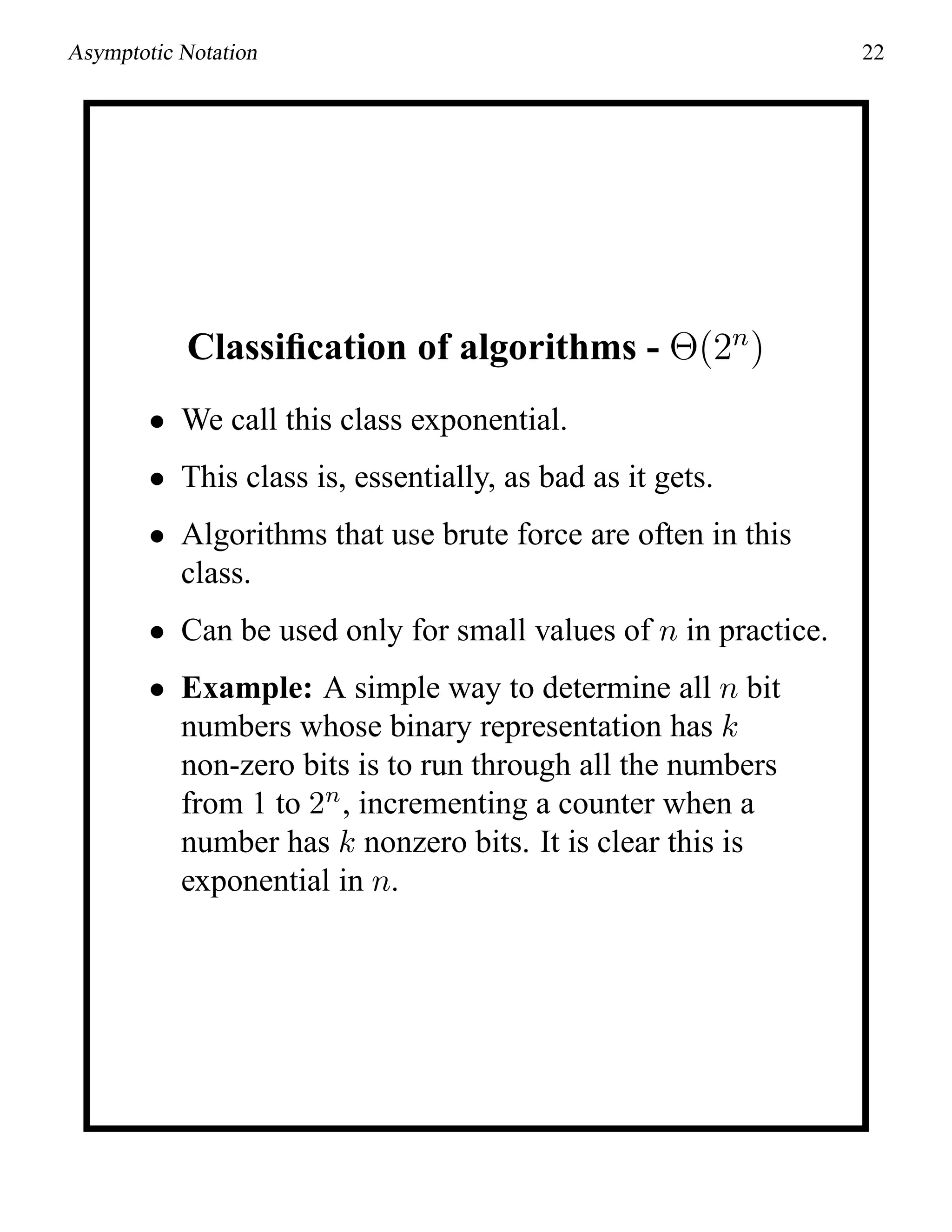
Classification of algorithms - Θ(1)
• Operations are performed k times, where k is
some constant, independent of the size of the
input n.
• This is the best one can hope for, and most often
unattainable.
• Examples:
int Fifth_Element(int A[],int n) {
return A[5];
}
int Partial_Sum(int A[],int n) {
int sum=0;
for(int i=0;i<42;i++)
sum=sum+A[i];
return sum;
}](https://image.slidesharecdn.com/asymptoticnotation-170214063057/75/Asymptotic-notation-17-2048.jpg)
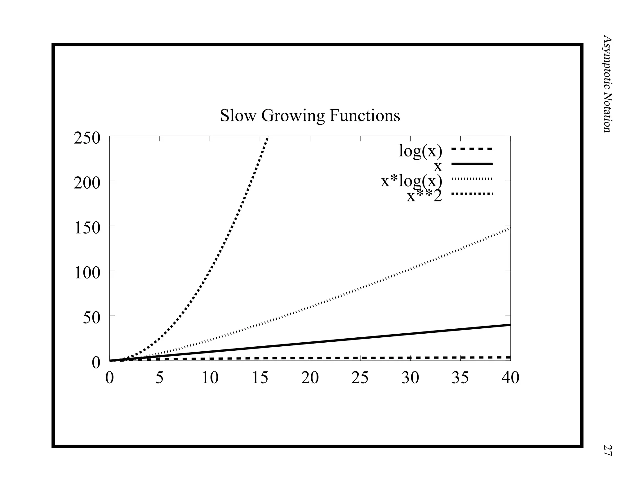
![Asymptotic Notation 19
Classification of algorithms - Θ(log n)
• A logarithmic function is the inverse of an
exponential function, i.e. bx
= n is equivalent to
x = logb n)
• Always increases, but at a slower rate as n
increases. (Recall that the derivative of log n is 1
n ,
a decreasing function.)
• Typically found where the algorithm can
systematically ignore fractions of the input.
• Examples:
int binarysearch(int a[], int n, int val)
{
int l=1, r=n, m;
while (r>=1) {
m = (l+r)/2;
if (a[m]==val) return m;
if (a[m]>val) r=m-1;
else l=m+1; }
return -1;
}](https://image.slidesharecdn.com/asymptoticnotation-170214063057/75/Asymptotic-notation-19-2048.jpg)
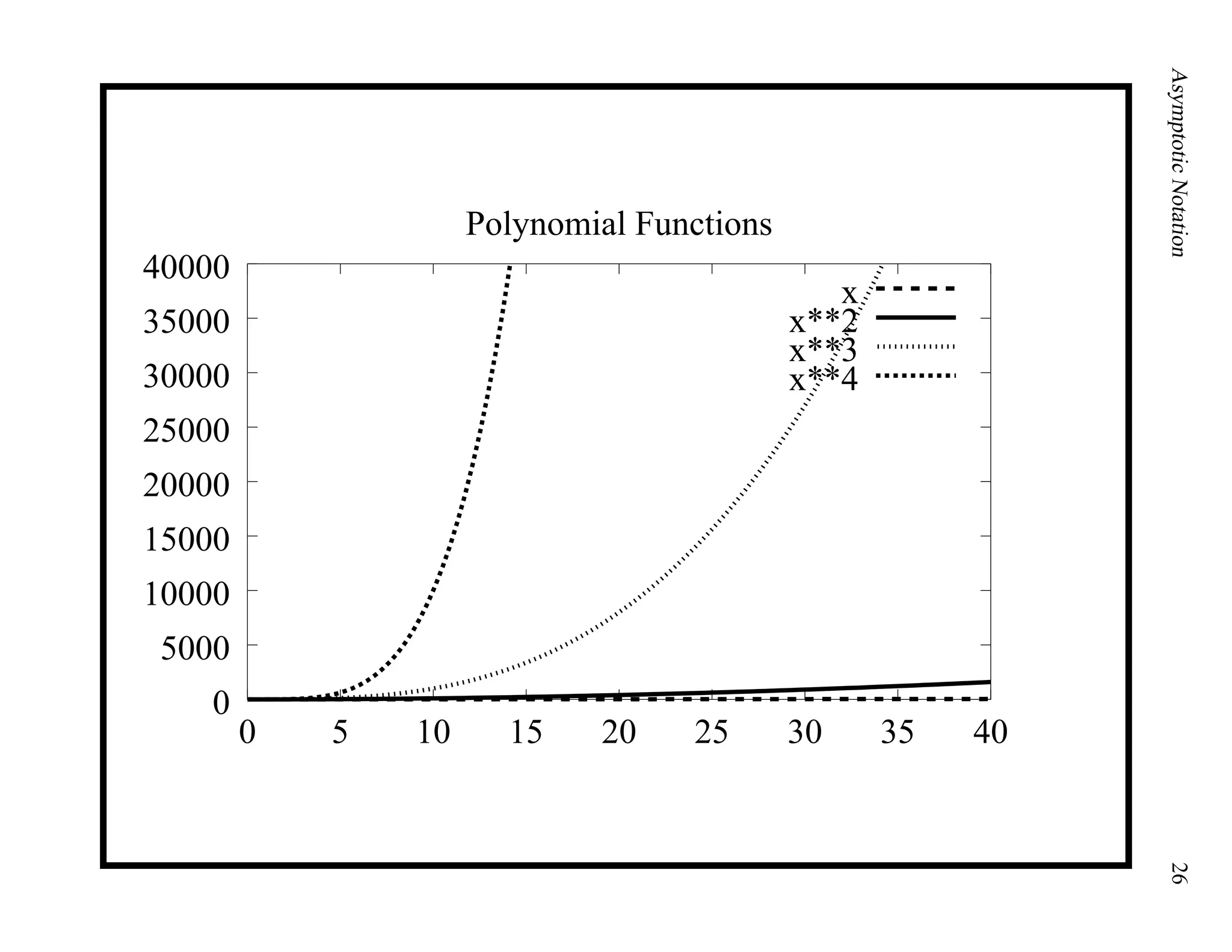
![Asymptotic Notation 21
Classification of algorithms - Θ(n2
)
• We call this class quadratic.
• As n doubles, run-time quadruples.
• However, it is still polynomial, which we consider
to be good.
• Typically found where algorithms deal with all
pairs of data.
• Example:
int *compute_sums(int A[], int n) {
int M[n][n];
int i,j;
for (i=0;i<n;i++)
for (j=0;j<n;j++)
M[i][j]=A[i]+A[j];
return M;
}
• More generally, if an algorithm is Θ(nk
) for
constant k it is called a polynomial-time
algorithm.](https://image.slidesharecdn.com/asymptoticnotation-170214063057/75/Asymptotic-notation-21-2048.jpg)
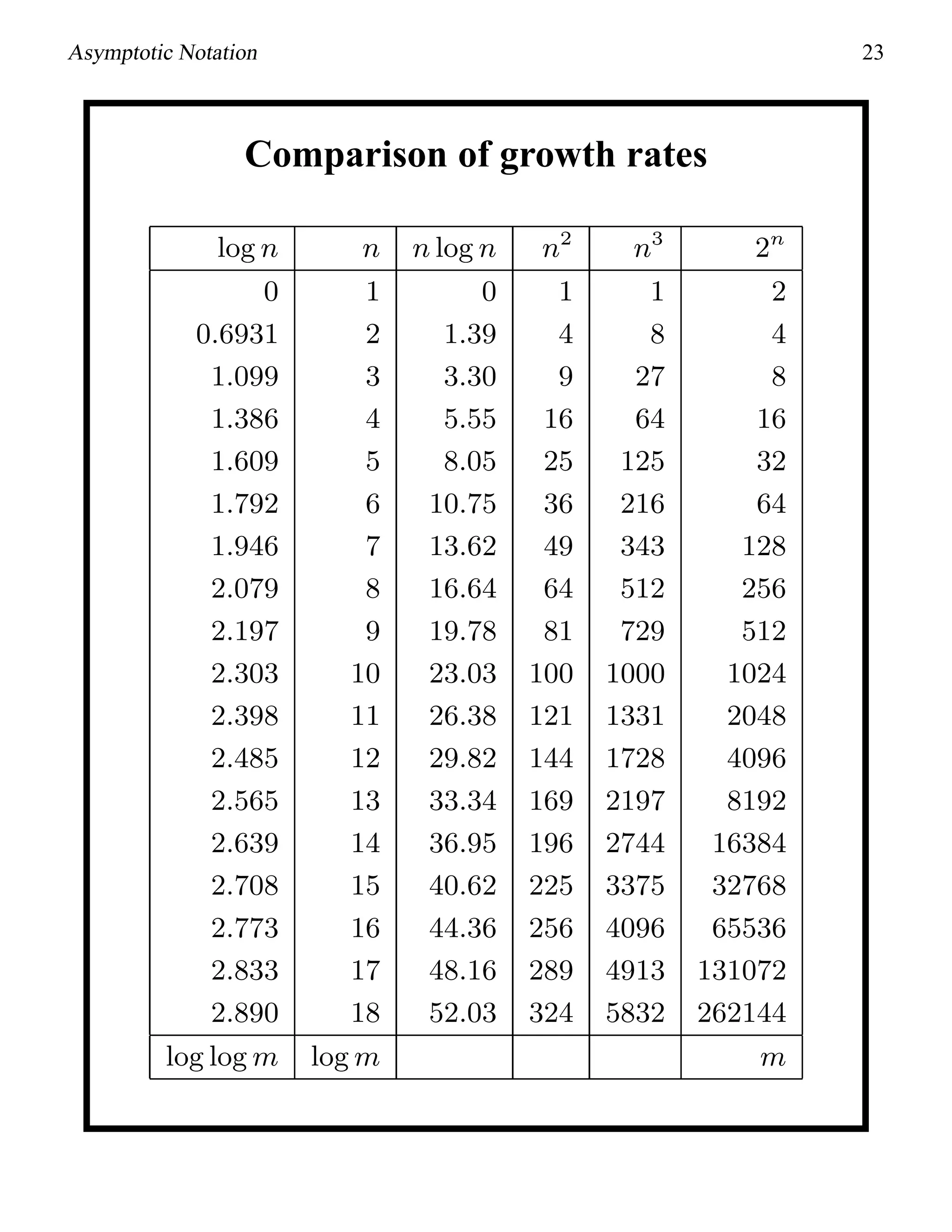
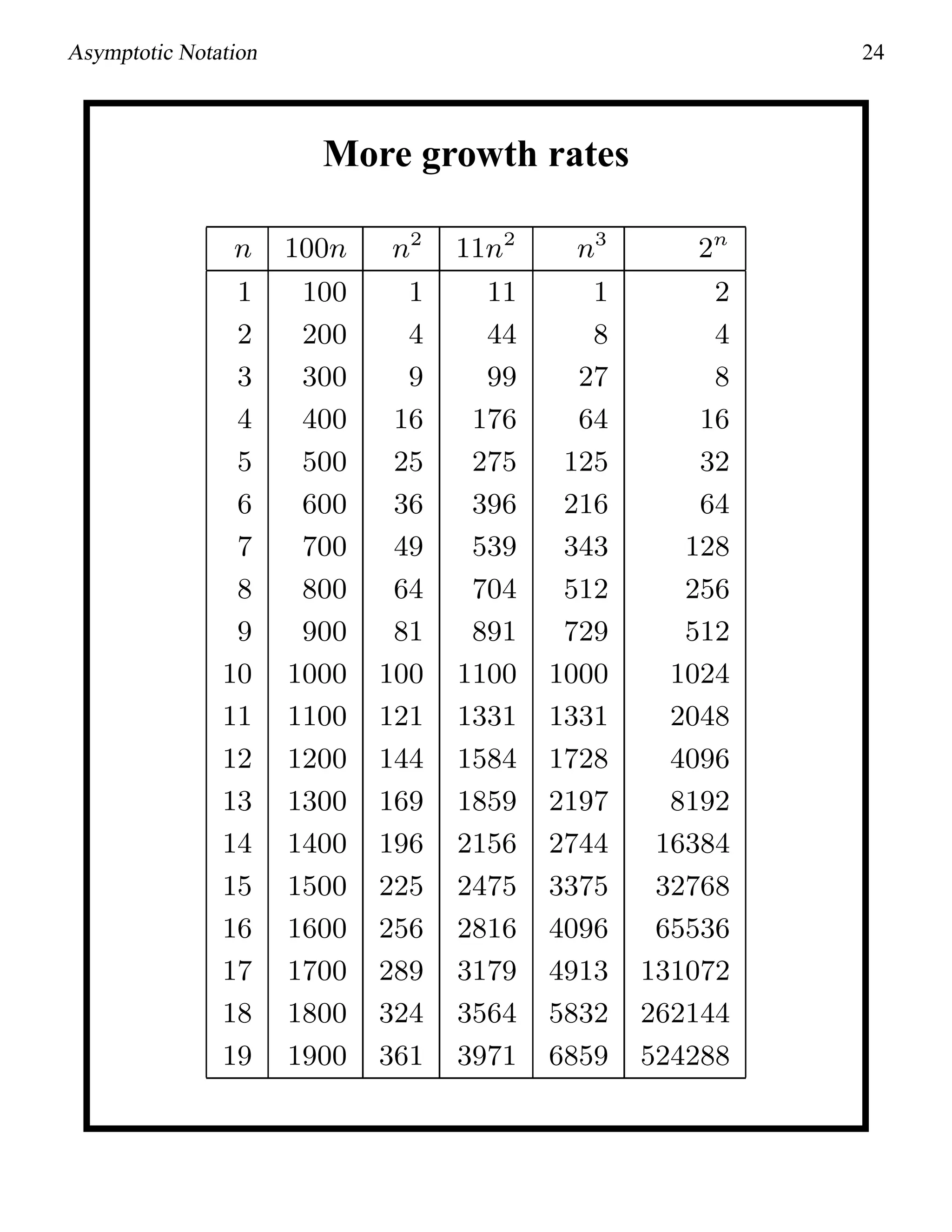
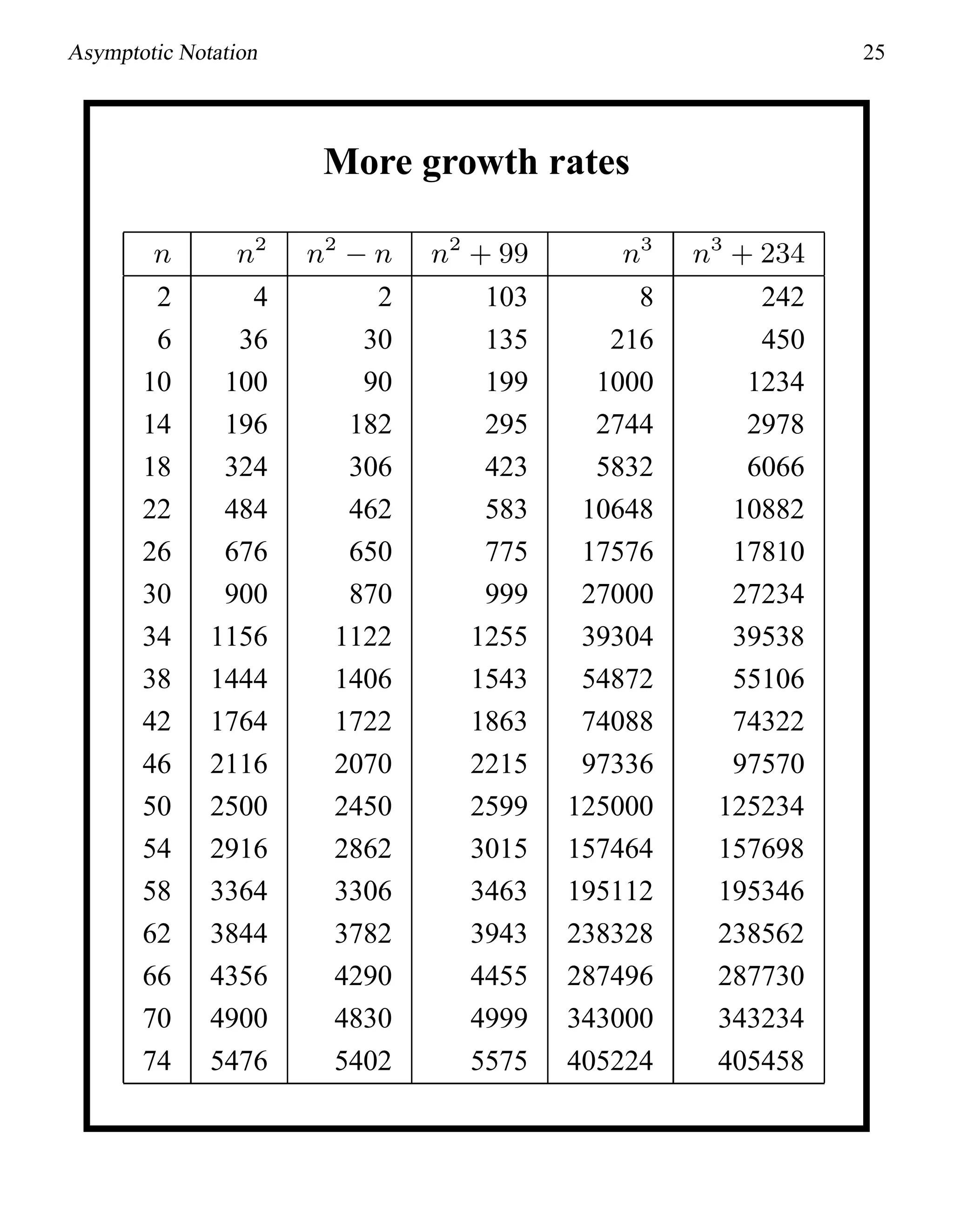
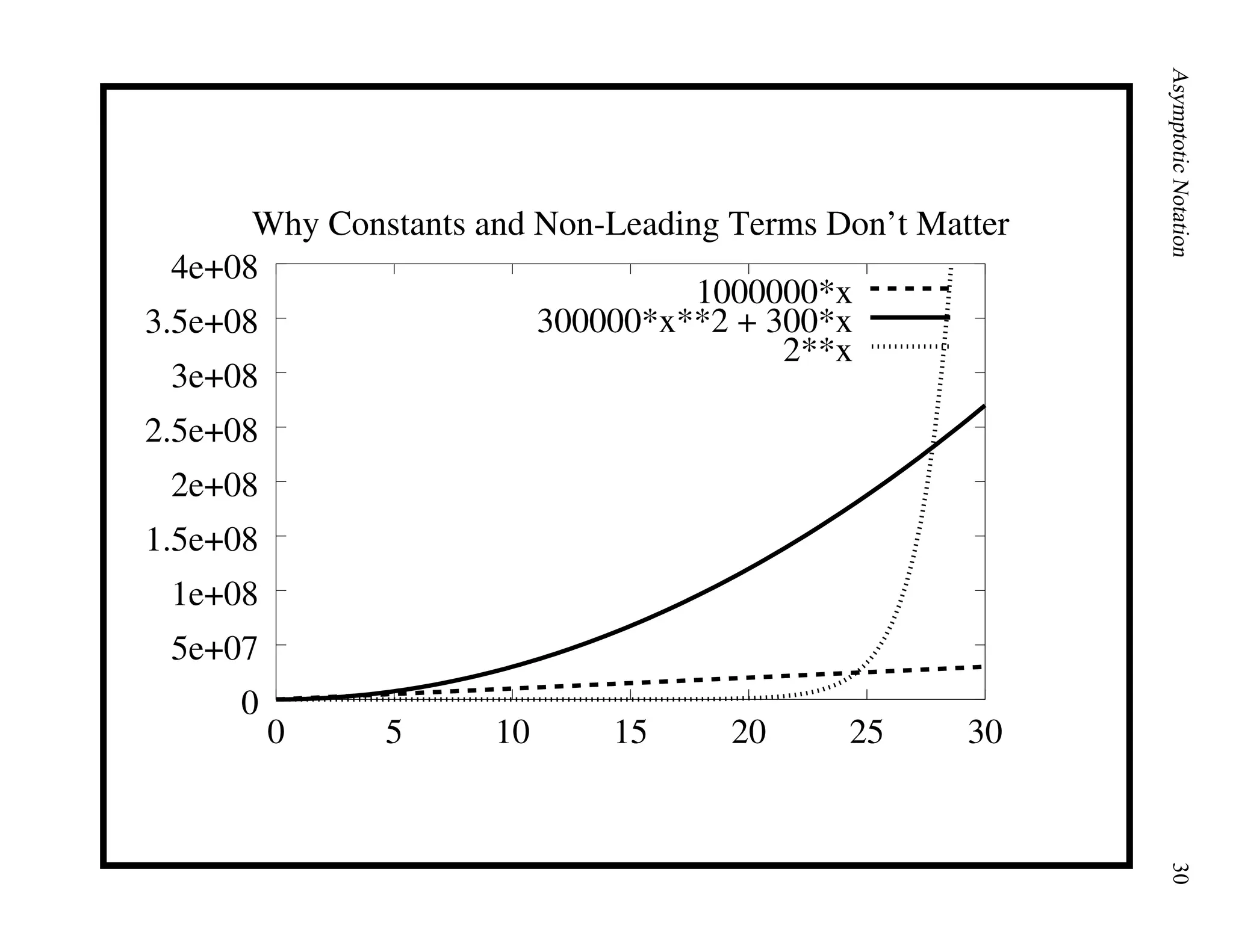
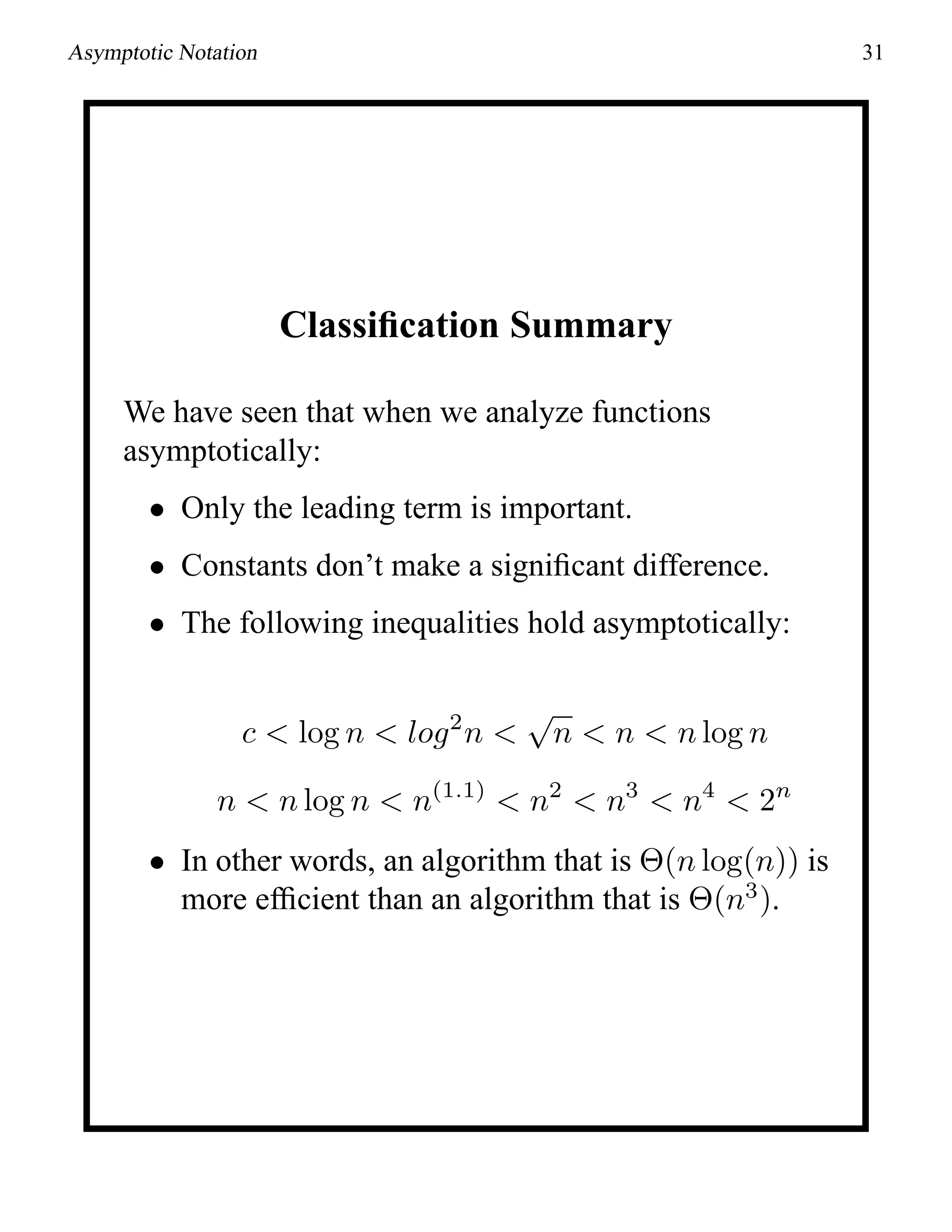

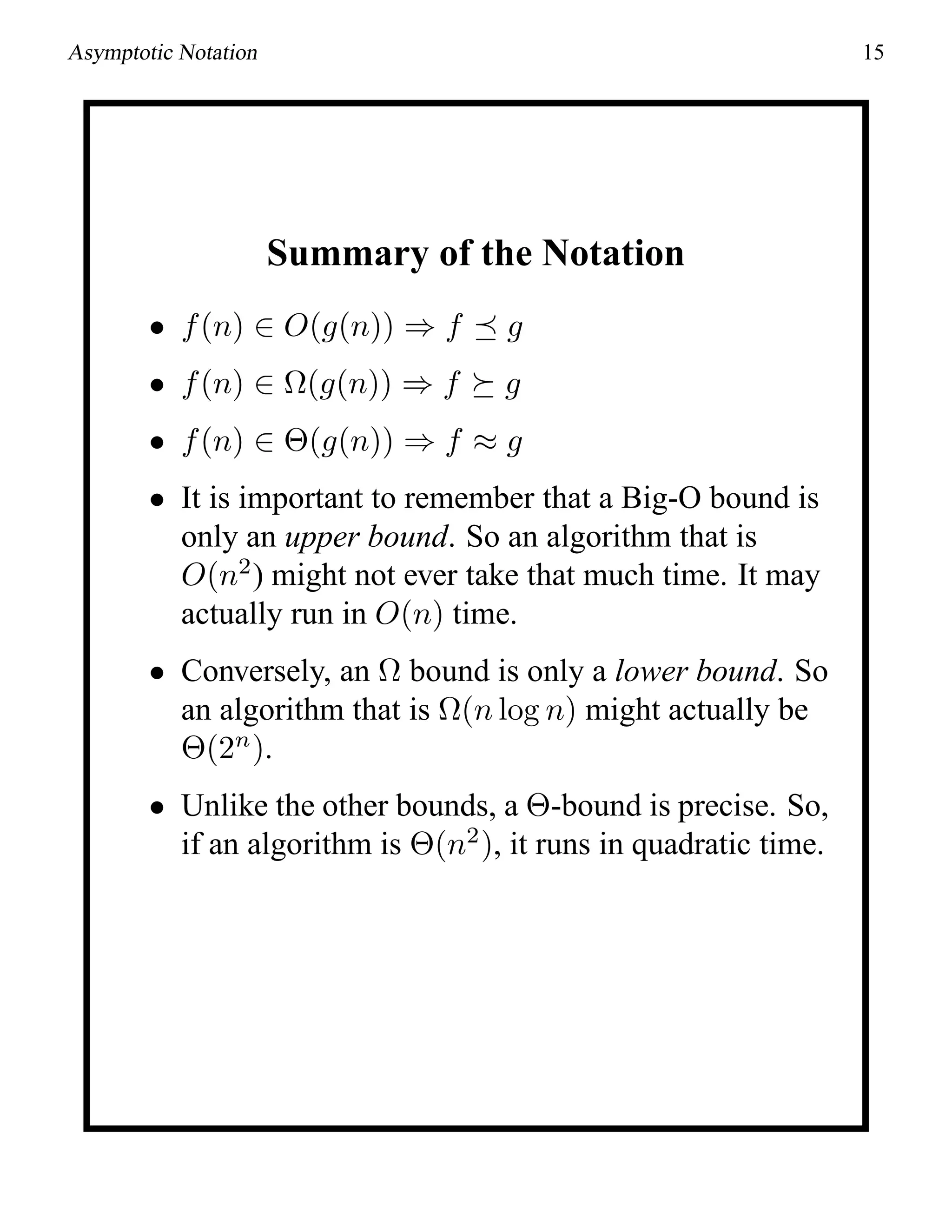
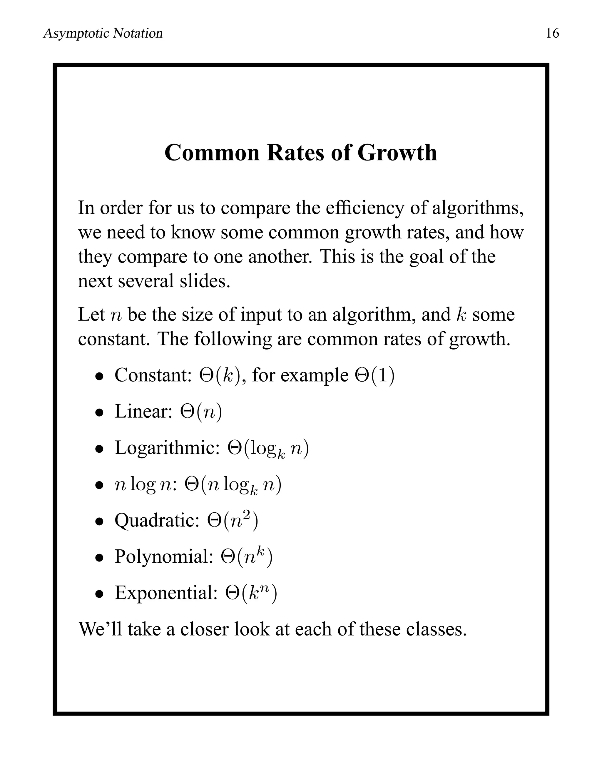
This document provides an introduction to asymptotic notation, which is used to classify algorithms according to their running time or space requirements. It defines common asymptotic notations like Big-O, Big-Omega, and Big-Theta and provides examples of algorithms that run in constant time (O(1)), linear time (O(n)), logarithmic time (O(log n)), quadratic time (O(n^2)), and other runtimes. The document also compares common growth rates like constant, linear, logarithmic, n log n, quadratic, polynomial, and exponential functions. Overall, it establishes the foundation for discussing the asymptotic efficiency of algorithms.