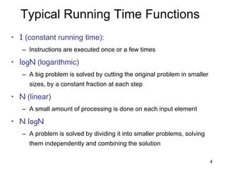
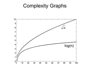
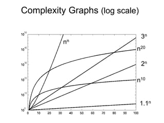
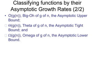
The document discusses algorithm analysis and asymptotic notation. It begins by explaining how to analyze algorithms to predict resource requirements like time and space. It defines asymptotic notation like Big-O, which describes an upper bound on the growth rate of an algorithm's running time. The document then provides examples of analyzing simple algorithms and classifying functions based on their asymptotic growth rates. It also introduces common time functions like constant, logarithmic, linear, quadratic, and exponential time and compares their growth.

1. CSE-245
Algorithms
Asymptotic Notation

2. 2
Analyzing Algorithms
• Predict the amount of resources required:
• memory: how much space is needed?
• computational time: how fast the algorithm runs?
• FACT: running time grows with the size of the input
• Input size (number of elements in the input)
– Size of an array, polynomial degree, # of elements in a matrix, # of bits in
the binary representation of the input, vertices and edges in a graph
Def: Running time = the number of primitive operations (steps) executed
before termination
– Arithmetic operations (+, -, *), data movement, control, decision making
(if, while), comparison

3. 3
Algorithm Analysis: Example
• Alg.: MIN (a[1], …, a[n])
m ← a[1];
for i ← 2 to n
if a[i] < m
then m ← a[i];
• Running time:
– the number of primitive operations (steps) executed
before termination
T(n) =1 [first step] + (n) [for loop] + (n-1) [if condition] +
(n-1) [the assignment in then] = 3n - 1
• Order (rate) of growth:
– The leading term of the formula
– Expresses the asymptotic behavior of the algorithm

4. 4
Typical Running Time Functions
• 1 (constant running time):
– Instructions are executed once or a few times
• logN (logarithmic)
– A big problem is solved by cutting the original problem in smaller
sizes, by a constant fraction at each step
• N (linear)
– A small amount of processing is done on each input element
• N logN
– A problem is solved by dividing it into smaller problems, solving
them independently and combining the solution

5. 5
Typical Running Time Functions
• N2 (quadratic)
– Typical for algorithms that process all pairs of data items (double
nested loops)
• N3 (cubic)
– Processing of triples of data (triple nested loops)
• NK (polynomial)
• 2N (exponential)
– Few exponential algorithms are appropriate for practical use

6. 6
Growth of Functions

7. Complexity Graphs
log(n)
n

8. Complexity Graphs
log(n)
n
n
n log(n)

9. Complexity Graphs
n10
n log(n)
n3
n2

10. Complexity Graphs (log scale)
n10
n20
nn
1.1n
2n
3n

11. Algorithm Complexity
• Worst Case Complexity:
– the function defined by the maximum number of steps
taken on any instance of size n
• Best Case Complexity:
– the function defined by the minimum number of steps
taken on any instance of size n
• Average Case Complexity:
– the function defined by the average number of steps
taken on any instance of size n

12. Best, Worst, and Average Case Complexity
Worst Case
Complexity
Average Case
Complexity
Best Case
Complexity
Number
of steps
N
(input size)

13. Doing the Analysis
• It’s hard to estimate the running time exactly
– Best case depends on the input
– Average case is difficult to compute
– So we usually focus on worst case analysis
• Easier to compute
• Usually close to the actual running time
• Strategy: find a function (an equation) that, for large n, is an
upper bound to the actual function (actual number of steps,
memory usage, etc.)
Upper bound
Lower bound
Actual function

14. Motivation for Asymptotic Analysis
• An exact computation of worst-case running time
can be difficult
– Function may have many terms:
• 4n2 - 3n log n + 17.5 n - 43 n⅔ + 75
• An exact computation of worst-case running time
is unnecessary
– Remember that we are already approximating running
time by using RAM model

15. Classifying functions by their
Asymptotic Growth Rates (1/2)
• asymptotic growth rate, asymptotic order, or
order of functions
– Comparing and classifying functions that ignores
• constant factors and
• small inputs.
• The Sets big oh O(g), big theta (g), big omega
(g)

16. Classifying functions by their
Asymptotic Growth Rates (2/2)
• O(g(n)), Big-Oh of g of n, the Asymptotic Upper
Bound;
 (g(n)), Theta of g of n, the Asymptotic Tight
Bound; and
 (g(n)), Omega of g of n, the Asymptotic Lower
Bound.

17. 17
Big-O
• What does it mean?
– If f(n) = O(n2), then:
• f(n) can be larger than n2 sometimes, but…
• We can choose some constant c and some value n0 such
that for every value of n larger than n0 : f(n) < cn2
• That is, for values larger than n0, f(n) is never more than a
constant multiplier greater than n2
• Or, in other words, f(n) does not grow more than a constant
factor faster than n2.
   
 
    0
0
all
for
0
such that
and
constants
positive
exist
there
:
n
n
n
cg
n
f
n
c
n
g
O
n
f





18. 18
Visualization of O(g(n))
n0
cg(n)
f(n)

19. 19
Examples
– 2n2 = O(n3):
– n2 = O(n2):
– 1000n2+1000n = O(n2):
– n = O(n2):
2n2 ≤ cn3  2 ≤ cn  c = 1 and n0= 2
n2 ≤ cn2  c ≥ 1  c = 1 and n0= 1
1000n2+1000n ≤ cn2 ≤ cn2+ 1000n  c=1001 and n0 = 1
n ≤ cn2  cn ≥ 1  c = 1 and n0= 1

20. 20
Big-O
 
 
 
 
 
2
1
.
2
2
3
2
2
2
2
2
2
2
2
20
7
5
000
,
150
000
,
000
,
1
2
n
O
n
n
O
n
n
O
n
n
n
O
n
n
O
n










21. 21
More Big-O
• Prove that:
• Let c = 21 and n0 = 4
• 21n2 > 20n2 + 2n + 5 for all n > 4
n2 > 2n + 5 for all n > 4
TRUE
 
2
2
5
2
20 n
O
n
n 



22. 22
Tight bounds
• We generally want the tightest bound we can
find.
• While it is true that n2 + 7n is in O(n3), it is more
interesting to say that it is in O(n2)

23. 23
Big Omega – Notation
• () – A lower bound
– n2 = (n)
– Let c = 1, n0 = 2
– For all n  2, n2 > 1  n
   
 
    0
0
all
for
0
such that
and
constants
positive
exist
there
:
n
n
n
cg
n
f
n
c
n
g
n
f






24. 24
Visualization of (g(n))
n0
cg(n)
f(n)

25. 25
-notation
• Big-O is not a tight upper bound. In other words
n = O(n2)
•  provides a tight bound
• In other words,
   
 
      0
2
1
0
2
1
all
for
0
such that
and
,
,
constants
positive
exist
there
:
n
n
n
g
c
n
f
n
g
c
n
c
c
n
g
n
f






   
     
     
 
n
g
n
f
n
g
O
n
f
n
g
n
f 




 AND

26. 26
Visualization of (g(n))
n0
c2g(n)
f(n)
c1g(n)

27. 27
A Few More Examples
• n = O(n2) ≠ (n2)
• 200n2 = O(n2) = (n2)
• n2.5 ≠ O(n2) ≠ (n2)

28. 28
Example 2
• Prove that:
• Let c = 21 and n0 = 10
• 21n3 > 20n3 + 7n + 1000 for all n > 10
n3 > 7n + 5 for all n > 10
TRUE, but we also need…
• Let c = 20 and n0 = 1
• 20n3 < 20n3 + 7n + 1000 for all n  1
TRUE
 
3
3
1000
7
20 n
n
n 




29. 29
Example 3
• Show that
• Let c = 2 and n0 = 5
 
n
n
n 2
O
2 2


 
5
2
1
2
2
2
2
2
2
2
2
2
2
2
2
1
2
1
2














n
n
n
n
n
n
n
n
n
n
n
n
n
n


30. 30
Asymptotic Notations - Examples
•  notation
– n2/2 – n/2
– (6n3 + 1)lgn/(n + 1)
– n vs. n2
•  notation
– n3 vs. n2
– n vs. logn
– n vs. n2
= (n2)
n ≠ (n2)
= (n2lgn)
• O notation
– 2n2 vs. n3
– n2 vs. n2
– n3 vs. nlogn
n3 = (n2)
n = (logn)
n  (n2)
2n2 = O(n3)
n2 = O(n2)
n3  O(nlgn)

31. 31
Asymptotic Notations - Examples
• For each of the following pairs of functions, either f(n) is
O(g(n)), f(n) is Ω(g(n)), or f(n) = Θ(g(n)). Determine
which relationship is correct.
– f(n) = log n2; g(n) = log n + 5
– f(n) = n; g(n) = log n2
– f(n) = log log n; g(n) = log n
– f(n) = n; g(n) = log2 n
– f(n) = n log n + n; g(n) = log n
– f(n) = 10; g(n) = log 10
– f(n) = 2n; g(n) = 10n2
– f(n) = 2n; g(n) = 3n
f(n) =  (g(n))
f(n) = (g(n))
f(n) = O(g(n))
f(n) = (g(n))
f(n) = (g(n))
f(n) = (g(n))
f(n) = (g(n))
f(n) = O(g(n))

32. 32
Simplifying Assumptions
• 1. If f(n) = O(g(n)) and g(n) = O(h(n)), then f(n) = O(h(n))
• 2. If f(n) = O(kg(n)) for any k > 0, then f(n) = O(g(n))
• 3. If f1(n) = O(g1(n)) and f2(n) = O(g2(n)),
• then f1(n) + f2(n) = O(max (g1(n), g2(n)))
• 4. If f1(n) = O(g1(n)) and f2(n) = O(g2(n)),
• then f1(n) * f2(n) = O(g1(n) * g2(n))

33. Example #1: carry n items
from one room to another room
• How many operations?
• n pick-ups, n forward moves, n drops and n
reverse moves  4 n operations
• 4n operations = c. n = O(c. n) = O(n)
• Similarly, any program that reads n inputs from
the user will have minimum time complexity
O(n).

34. Example #2: Locating patient record in
Doctor Office
What is the time complexity of search?
• Binary Search algorithm at work
• O(log n)
• Sequential search?
• O(n)

35. Example #3: Store manager gives gifts
to first 10 customers
• There are n customers in the queue.
• Manager brings one gift at a time.
• Time complexity = O(c. 10) = O(1)
• Manager will take exactly same time irrespective
of the line length.

36. 36
Loops with Break
for (j = 0; j < n; ++j) {
// 3 atomics
if (condition) break;
}
• Upper bound = O(4n) = O(n)
• Lower bound = Ω(4) = Ω(1)
• Complexity = O(n)
Home Work Ques: Why don’t we have a (…)
notation here?

37. 37
Sequential Search
• Given an unsorted vector/list a[ ], find the
location of element X.
for (i = 0; i < n; i++) {
if (a[i] == X) return true;
}
return false;
• Input size: n = array size()
• Complexity = O(n)

38. 38
If-then-else Statement
• Complexity = ??
= O(1) + max ( O(1), O(N))
= O(1) + O(N)
= O(N)
if(condition)
i = 0;
else
for ( j = 0; j < n; j++)
a[j] = j;

39. 39
Consecutive Statements
• Add the complexity of consecutive statements
• Complexity = (3n + 5n) = (n)
for (j = 0; j < n; ++j) {
// 3 atomics
}
for (j = 0; j < n; ++j) {
// 5 atomics
}

40. 40
Nested Loop Statements
• Analyze such statements inside out
for (j = 0; j < n; ++j) {
// 2 atomics
for (k = 0; k < n; ++k) {
// 3 atomics
}
}
• Complexity = ((2 + 3n)n) = (n2)

41. 41
Recursion
long factorial( int n )
{
if( n <= 1 )
return 1;
else
return n*factorial(n- 1);
}
In terms of big-Oh:
t(1) = 1
t(n) = 1 + t(n-1) = 1 + 1 + t(n-2)
= ... k + t(n-k)
Choose k = n-1
t(n) = n-1 + t(1) = n-1 + 1 = O(n)
Consider the following time complexity:
t(0) = 1
t(n) = 1 + 2t(n-1) = 1 + 2(1 + 2t(n-2)) = 1 + 2 + 4t(n-2)
= 1 + 2 + 4(1 + 2t(n-3)) = 1 + 2 + 4 + 8t(n-3)
= 1 + 2 + ... + 2k-1 + 2kt(n-k)
Choose k = n
t(n) - 1 + 2 + ... 2n-1 + 2n = 2n+1 - 1

42. 42
Binary Search
• Given a sorted vector/list a[ ], find the location of element X
unsigned int binary_search(vector<int> a, int X)
{
unsigned int low = 0, high = a.size()-1;
while (low <= high) {
int mid = (low + high) / 2;
if (a[mid] < X)
low = mid + 1;
else if( a[mid] > X )
high = mid - 1;
else
return mid;
}
return NOT_FOUND;
}
• Input size: n = array size()
• Complexity = O( k iterations x (1 comparison+1 assignment) per loop)
= O(log(n))

43. 43
Example
• Code:
• a = b;
• Complexity:

44. 44
Example
• Code:
• sum = 0;
• for (i=1; i <=n; i++)
• sum += n;
• Complexity:

45. 45
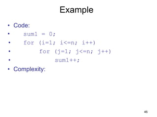
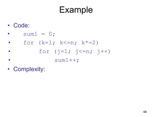
Example
• Code:
• sum = 0;
• for (j=1; j<=n; j++)
• for (i=1; i<=j; i++)
• sum++;
• for (k=0; k<n; k++)
• A[k] = k;
• Complexity:

46. 46
Example
• Code:
• sum1 = 0;
• for (i=1; i<=n; i++)
• for (j=1; j<=n; j++)
• sum1++;
• Complexity:

47. 47
Example
• Code:
• sum2 = 0;
• for (i=1; i<=n; i++)
• for (j=1; j<=i; j++)
• sum2++;
• Complexity:

48. 48
Example
• Code:
• sum1 = 0;
• for (k=1; k<=n; k*=2)
• for (j=1; j<=n; j++)
• sum1++;
• Complexity:

49. 49
Example
• Code:
• sum2 = 0;
• for (k=1; k<=n; k*=2)
• for (j=1; j<=k; j++)
• sum2++;
• Complexity:

50. Summary
• Time complexity is a measure of algorithm
efficiency
• Efficient algorithm plays the major role in
determining the running time.
Q: Is it possible to determine running time based
on algorithm’s time complexity alone?
• Minor tweaks in the code can cut down the
running time by a factor too.
• Other items like CPU speed, memory speed,
device I/O speed can help as well.
• For certain problems, it is possible to allocate
additional space & improve time complexity.

51. Summary
• Time complexity is a measure of algorithm
efficiency
• Efficient algorithm plays the major role in
determining the running time.
Q: Is it possible to determine running time based
on algorithm’s time complexity alone?
• Minor tweaks in the code can cut down the
running time by a factor too.
• Other items like CPU speed, memory speed,
device I/O speed can help as well.
• For certain problems, it is possible to allocate
additional space & improve time complexity.