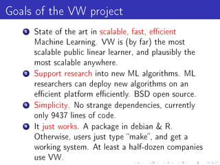
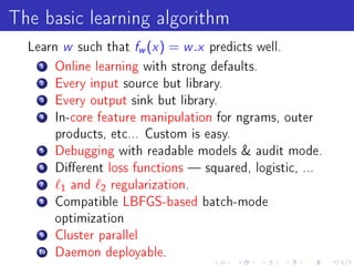
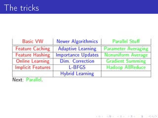
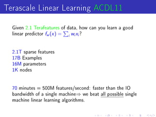
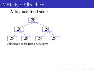
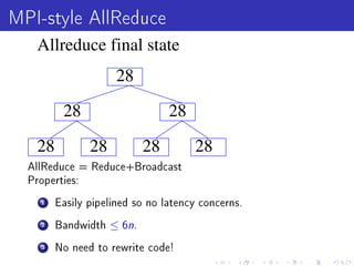
Vowpal Wabbit is a machine learning system that has four main goals: scalable and efficient machine learning, supporting new algorithm research, simplicity with few dependencies, and usability with minimal setup requirements. It uses several "tricks" like feature hashing and caching, online learning, and importance weighting to achieve scalability. It also supports newer algorithms like adaptive learning rates and dimensional correction. Vowpal Wabbit can be run in parallel on large clusters to handle terascale problems with billions of examples.

1. Technical Tricks of Vowpal Wabbit
http://hunch.net/~vw/
John Langford, Columbia, Data-Driven Modeling,
April 16
git clone
git://github.com/JohnLangford/vowpal_wabbit.git

2. Goals of the VW project
1 State of the art in scalable, fast, ecient
Machine Learning. VW is (by far) the most
scalable public linear learner, and plausibly the
most scalable anywhere.
2 Support research into new ML algorithms. ML
researchers can deploy new algorithms on an
ecient platform eciently. BSD open source.
3 Simplicity. No strange dependencies, currently
only 9437 lines of code.
4 It just works. A package in debian R.
Otherwise, users just type make, and get a
working system. At least a half-dozen companies
use VW.

3. Demonstration
vw -c rcv1.train.vw.gz exact_adaptive_norm
power_t 1 -l 0.5

4. The basic learning algorithm
Learn w such that fw (x ) = w .x predicts well.
1 Online learning with strong defaults.
2 Every input source but library.
3 Every output sink but library.
4 In-core feature manipulation for ngrams, outer
products, etc... Custom is easy.
5 Debugging with readable models audit mode.
6 Dierent loss functions squared, logistic, ...
7
1 and 2 regularization.
8 Compatible LBFGS-based batch-mode
optimization
9 Cluster parallel
10 Daemon deployable.

5. The tricks
Basic VW Newer Algorithmics Parallel Stu
Feature Caching Adaptive Learning Parameter Averaging
Feature Hashing Importance Updates Nonuniform Average
Online Learning Dim. Correction Gradient Summing
Implicit Features L-BFGS Hadoop AllReduce
Hybrid Learning
We'll discuss Basic VW and algorithmics, then Parallel.

6. Feature Caching
Compare: time vw rcv1.train.vw.gz exact_adaptive_norm
power_t 1

7. Feature Hashing
String − Index dictionary
RAM
Weights Weights
Conventional VW
Most algorithms use a hashmap to change a word into an
index for a weight.
VW uses a hash function which takes almost no RAM, is x10
faster, and is easily parallelized.

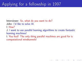
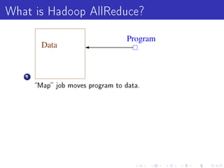
8. The spam example [WALS09]
1 3.2 ∗ 106 labeled emails.
2 433167 users.
3 ∼ 40 ∗ 106 unique features.
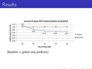
How do we construct a spam lter which is personalized, yet
uses global information?

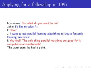
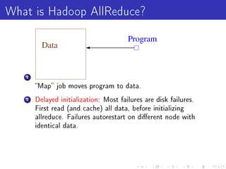
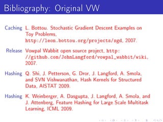
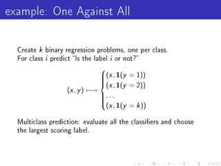
9. The spam example [WALS09]
1 3.2 ∗ 106 labeled emails.
2 433167 users.
3 ∼ 40 ∗ 106 unique features.
How do we construct a spam lter which is personalized, yet
uses global information?
Answer: Use hashing to predict according to:
w , φ(x ) + w , φ (x )
u

10. Results
(baseline = global only predictor)

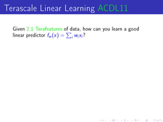
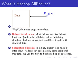
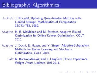
11. Basic Online Learning
Start with ∀i : w
i = 0, Repeatedly:
1 Get example x ∈ (∞, ∞)∗.
2 Make prediction y −
ˆ w x clipped to interval [0, 1].
i i i
3 Learn truth y ∈ [0, 1] with importance I or goto (1).
4 Update w ← w + η 2(y − y )Ix and go to (1).
i i ˆ i

12. Reasons for Online Learning
1 Fast convergence to a good predictor
2 It's RAM ecient. You need store only one example in
RAM rather than all of them. ⇒ Entirely new scales of
data are possible.
3 Online Learning algorithm = Online Optimization
Algorithm. Online Learning Algorithms ⇒ the ability to
solve entirely new categories of applications.
4 Online Learning = ability to deal with drifting
distributions.

13. Implicit Outer Product
Sometimes you care about the interaction of two sets of
features (ad features x query features, news features x user
features, etc...).
Choices:
1 Expand the set of features explicitly, consuming n2 disk
space.
2 Expand the features dynamically in the core of your
learning algorithm.

14. Implicit Outer Product
Sometimes you care about the interaction of two sets of
features (ad features x query features, news features x user
features, etc...).
Choices:
1 Expand the set of features explicitly, consuming n2 disk
space.
2 Expand the features dynamically in the core of your
learning algorithm.
Option (2) is x10 faster. You need to be comfortable with
hashes rst.

15. The tricks
Basic VW Newer Algorithmics Parallel Stu
Feature Caching Adaptive Learning Parameter Averaging
Feature Hashing Importance Updates Nonuniform Average
Online Learning Dim. Correction Gradient Summing
Implicit Features L-BFGS Hadoop AllReduce
Hybrid Learning
Next: algorithmics.

16. Adaptive Learning [DHS10,MS10]
For example t , let g it = 2(y − y )xit .
ˆ

17. Adaptive Learning [DHS10,MS10]
For example t , let g it = 2(y − y )xit .
ˆ
New update rule: w i ← wi − η √Pit,t +1
g
2
t =1 git

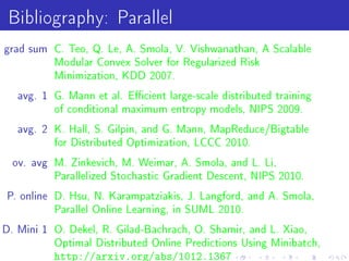
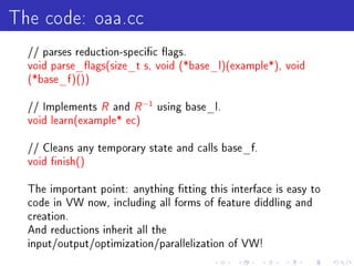
18. Adaptive Learning [DHS10,MS10]
For example t , let g it = 2(y − y )xit .
ˆ
New update rule: w i ← wi − η √Pit,t +1
g
2
t =1 git
Common features stabilize quickly. Rare features can have
large updates.

19. Learning with importance weights [KL11]
y

20. Learning with importance weights [KL11]
wt x y

21. Learning with importance weights [KL11]
−η( ) x
wt x y

22. Learning with importance weights [KL11]
−η( ) x
wt x wt+1 x y

23. Learning with importance weights [KL11]
−6η( ) x
wt x y

24. Learning with importance weights [KL11]
−6η( ) x
wt x y wt+1 x ??

25. Learning with importance weights [KL11]
−η( ) x
wt x y wt+1 x

26. Learning with importance weights [KL11]
wt x wt+1 x y

27. Learning with importance weights [KL11]
s(h)||x||2
wt x wt+1 x y

28. Robust results for unweighted problems
astro - logistic loss spam - quantile loss
0.97 0.98
0.96 0.97
0.96
0.95
0.95
standard
standard
0.94
0.94
0.93
0.93
0.92
0.92
0.91 0.91
0.9 0.9
0.9 0.91 0.92 0.93 0.94 0.95 0.96 0.97 0.9 0.91 0.92 0.93 0.94 0.95 0.96 0.97 0.98
importance aware importance aware
rcv1 - squared loss webspam - hinge loss
0.95 1
0.945 0.99
0.94 0.98
0.935 0.97
0.93 0.96
standard
standard
0.925 0.95
0.92 0.94
0.915 0.93
0.91 0.92
0.905 0.91
0.9 0.9
0.9 0.905 0.91 0.915 0.92 0.925 0.93 0.935 0.94 0.945 0.95 0.9 0.91 0.92 0.93 0.94 0.95 0.96 0.97 0.98 0.99
importance aware importance aware

29. Dimensional Correction
Gradient of squared loss =
∂(fw (x )−y )2
∂ wi
f x
= 2( w ( ) − y )x i and
change weights in the negative gradient direction:
∂(fw (x ) − y )2
w i ← wi − η
∂ wi

30. Dimensional Correction
Gradient of squared loss =
∂(fw (x )−y )2
∂ wi
= 2( w ( ) − f x y )x i and
change weights in the negative gradient direction:
∂(fw (x ) − y )2
w i ← wi − η
∂ wi
But the gradient has intrinsic problems. w naturally has units
i
of 1/i since doubling x implies halving w to get the same
i i
prediction.
⇒ Update rule has mixed units!

31. Dimensional Correction
Gradient of squared loss =
∂(fw (x )−y )2
∂ wi
= 2( w ( ) − f x y )x i and
change weights in the negative gradient direction:
∂(fw (x ) − y )2
wi ← wi − η
∂ wi
But the gradient has intrinsic problems. w naturally has unitsi
of 1/i since doubling x implies halving w to get the same
i i
prediction.
⇒ Update rule has mixed units!
A crude x: divide update by x 2.
It helps much!
i i
(fw (x )−y )2
This is scary! The problem optimized is minw P 2
x ,y
i xi
rather than minw x ,y
(fw (x ) − y )2 . But it works.

32. LBFGS [Nocedal80]
Batch(!) second order algorithm. Core idea = ecient
approximate Newton step.

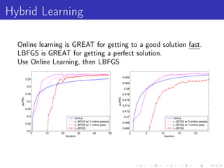
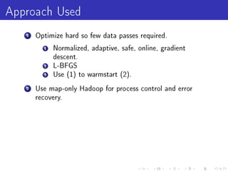
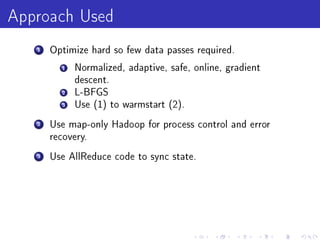
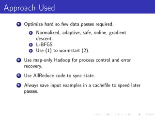
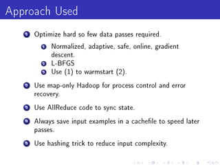
33. LBFGS [Nocedal80]
Batch(!) second order algorithm. Core idea = ecient
approximate Newton step.
H = ∂ (∂w (i ∂)−j )
2 f x y
2
= Hessian.
w w
Newton step = w → w + H −1g .

34. LBFGS [Nocedal80]
Batch(!) second order algorithm. Core idea = ecient
approximate Newton step.
H = ∂ (∂w (i ∂)−j )
2 f x y
2
= Hessian.
w w
Newton step = w → w + H −1g .
Newton fails: you can't even represent H.
Instead build up approximate inverse Hessian according to:
∆w ∆Tw where ∆ is a change in weights
∆T ∆g
w w w
and ∆g is a change
in the loss gradient g.

35. Hybrid Learning
Online learning is GREAT for getting to a good solution fast.
LBFGS is GREAT for getting a perfect solution.

36. Hybrid Learning
Online learning is GREAT for getting to a good solution fast.
LBFGS is GREAT for getting a perfect solution.
Use Online Learning, then LBFGS
0.484
0.55
0.482
0.5
0.48
0.45 0.478
auPRC
auPRC
0.476
0.4
0.474
0.35
0.472
0.3 0.47
Online Online
L−BFGS w/ 5 online passes 0.468 L−BFGS w/ 5 online passes
0.25 L−BFGS w/ 1 online pass L−BFGS w/ 1 online pass
L−BFGS 0.466 L−BFGS
0.2
0 10 20 30 40 50 0 5 10 15 20
Iteration Iteration

37. The tricks
Basic VW Newer Algorithmics Parallel Stu
Feature Caching Adaptive Learning Parameter Averaging
Feature Hashing Importance Updates Nonuniform Average
Online Learning Dim. Correction Gradient Summing
Implicit Features L-BFGS Hadoop AllReduce
Hybrid Learning
Next: Parallel.

38. Applying for a fellowship in 1997

39. Applying for a fellowship in 1997
Interviewer: So, what do you want to do?

40. Applying for a fellowship in 1997
Interviewer: So, what do you want to do?
John: I'd like to solve AI.

41. Applying for a fellowship in 1997
Interviewer: So, what do you want to do?
John: I'd like to solve AI.
I: How?

42. Applying for a fellowship in 1997
Interviewer: So, what do you want to do?
John: I'd like to solve AI.
I: How?
J: I want to use parallel learning algorithms to create fantastic
learning machines!

43. Applying for a fellowship in 1997
Interviewer: So, what do you want to do?
John: I'd like to solve AI.
I: How?
J: I want to use parallel learning algorithms to create fantastic
learning machines!
I: You fool! The only thing parallel machines are good for is
computational windtunnels!

44. Applying for a fellowship in 1997
Interviewer: So, what do you want to do?
John: I'd like to solve AI.
I: How?
J: I want to use parallel learning algorithms to create fantastic
learning machines!
I: You fool! The only thing parallel machines are good for is
computational windtunnels!
The worst part: he had a point.

45. Terascale Linear Learning ACDL11
Given 2.1 Terafeatures of data, how can you learn a good
linear predictor f (x ) =
w i
wx?
i i

46. Terascale Linear Learning ACDL11
Given 2.1 Terafeatures of data, how can you learn a good
linear predictor f (x ) =
w i
wx?
i i
2.1T sparse features
17B Examples
16M parameters
1K nodes

47. Terascale Linear Learning ACDL11
Given 2.1 Terafeatures of data, how can you learn a good
linear predictor f (x ) =
w i
wx?
i i
2.1T sparse features
17B Examples
16M parameters
1K nodes
70 minutes = 500M features/second: faster than the IO
bandwidth of a single machine⇒ we beat all possible single
machine linear learning algorithms.

48. Features/s
100
1000
10000
100000
1e+06
1e+07
1e+08
RBF-SVM 1e+09
MPI?-500
RCV1
Ensemble Tree
MPI-128
Synthetic
single
parallel
RBF-SVM
TCP-48
Parallel Learning book
MNIST 220K
Decision Tree
MapRed-200
Ad-Bounce #
Boosted DT
MPI-32
Speed per method
Ranking #
Linear
Threads-2
RCV1
Linear
adoop+TCP-1000
Ads *
Compare: Other Supervised Algorithms in

49. MPI-style AllReduce
Allreduce initial state
5 7 6
1 2 3 4

50. MPI-style AllReduce
Allreduce final state
28 28 28
28 28 28 28

51. MPI-style AllReduce
Create Binary Tree
7
5 6
1 2 3 4

52. MPI-style AllReduce
Reducing, step 1
7
8 13
1 2 3 4

53. MPI-style AllReduce
Reducing, step 2
28
8 13
1 2 3 4

54. MPI-style AllReduce
Broadcast, step 1
28
28 28
1 2 3 4

55. MPI-style AllReduce
Allreduce final state
28
28 28
28 28 28 28
AllReduce = Reduce+Broadcast

56. MPI-style AllReduce
Allreduce final state
28
28 28
28 28 28 28
AllReduce = Reduce+Broadcast
Properties:
1 Easily pipelined so no latency concerns.
2 Bandwidth ≤ 6n .
3 No need to rewrite code!

57. An Example Algorithm: Weight averaging
n = AllReduce(1)
While (pass number max)
1 While (examples left)
1 Do online update.
2 AllReduce(weights)
3 For each weight w ← w /n

58. An Example Algorithm: Weight averaging
n = AllReduce(1)
While (pass number max)
1 While (examples left)
1 Do online update.
2 AllReduce(weights)
3 For each weight w ← w /n
Other algorithms implemented:
1 Nonuniform averaging for online learning
2 Conjugate Gradient
3 LBFGS

59. What is Hadoop AllReduce?
Program
Data
1
Map job moves program to data.

60. What is Hadoop AllReduce?
Program
Data
1
Map job moves program to data.
2 Delayed initialization: Most failures are disk failures.
First read (and cache) all data, before initializing
allreduce. Failures autorestart on dierent node with
identical data.

61. What is Hadoop AllReduce?
Program
Data
1
Map job moves program to data.
2 Delayed initialization: Most failures are disk failures.
First read (and cache) all data, before initializing
allreduce. Failures autorestart on dierent node with
identical data.
3 Speculative execution: In a busy cluster, one node is
often slow. Hadoop can speculatively start additional
mappers. We use the rst to nish reading all data once.

62. Approach Used
1 Optimize hard so few data passes required.
1 Normalized, adaptive, safe, online, gradient
descent.
2 L-BFGS
3 Use (1) to warmstart (2).

63. Approach Used
1 Optimize hard so few data passes required.
1 Normalized, adaptive, safe, online, gradient
descent.
2 L-BFGS
3 Use (1) to warmstart (2).
2 Use map-only Hadoop for process control and error
recovery.

64. Approach Used
1 Optimize hard so few data passes required.
1 Normalized, adaptive, safe, online, gradient
descent.
2 L-BFGS
3 Use (1) to warmstart (2).
2 Use map-only Hadoop for process control and error
recovery.
3 Use AllReduce code to sync state.

65. Approach Used
1 Optimize hard so few data passes required.
1 Normalized, adaptive, safe, online, gradient
descent.
2 L-BFGS
3 Use (1) to warmstart (2).
2 Use map-only Hadoop for process control and error
recovery.
3 Use AllReduce code to sync state.
4 Always save input examples in a cachele to speed later
passes.

66. Approach Used
1 Optimize hard so few data passes required.
1 Normalized, adaptive, safe, online, gradient
descent.
2 L-BFGS
3 Use (1) to warmstart (2).
2 Use map-only Hadoop for process control and error
recovery.
3 Use AllReduce code to sync state.
4 Always save input examples in a cachele to speed later
passes.
5 Use hashing trick to reduce input complexity.

67. Approach Used
1 Optimize hard so few data passes required.
1 Normalized, adaptive, safe, online, gradient
descent.
2 L-BFGS
3 Use (1) to warmstart (2).
2 Use map-only Hadoop for process control and error
recovery.
3 Use AllReduce code to sync state.
4 Always save input examples in a cachele to speed later
passes.
5 Use hashing trick to reduce input complexity.
Open source in Vowpal Wabbit 6.1. Search for it.

68. Robustness Speedup
Speed per method
10
Average_10
9 Min_10
8 Max_10
linear
7
Speedup
6
5
4
3
2
1
0
10 20 30 40 50 60 70 80 90 100
Nodes

69. Splice Site Recognition
0.55
0.5
0.45
auPRC
0.4
0.35
0.3
Online
L−BFGS w/ 5 online passes
0.25 L−BFGS w/ 1 online pass
L−BFGS
0.2
0 10 20 30 40 50
Iteration

70. Splice Site Recognition
0.6
0.5
0.4
auPRC
0.3
0.2
L−BFGS w/ one online pass
0.1 Zinkevich et al.
Dekel et al.
0
0 5 10 15 20
Effective number of passes over data

71. To learn more
The wiki has tutorials, examples, and help:
https://github.com/JohnLangford/vowpal_wabbit/wiki
Mailing List: vowpal_wabbit@yahoo.com
Various discussion: http://hunch.net Machine Learning
(Theory) blog

72. Bibliography: Original VW
Caching L. Bottou. Stochastic Gradient Descent Examples on
Toy Problems,
http://leon.bottou.org/projects/sgd, 2007.
http:
Release Vowpal Wabbit open source project,
//github.com/JohnLangford/vowpal_wabbit/wiki,
2007.
Hashing Q. Shi, J. Petterson, G. Dror, J. Langford, A. Smola,
and SVN Vishwanathan, Hash Kernels for Structured
Data, AISTAT 2009.
Hashing K. Weinberger, A. Dasgupta, J. Langford, A. Smola, and
J. Attenberg, Feature Hashing for Large Scale Multitask
Learning, ICML 2009.

73. Bibliography: Algorithmics
L-BFGS J. Nocedal, Updating Quasi-Newton Matrices with
Limited Storage, Mathematics of Computation
35:773782, 1980.
Adaptive H. B. McMahan and M. Streeter, Adaptive Bound
Optimization for Online Convex Optimization, COLT
2010.
Adaptive J. Duchi, E. Hazan, and Y. Singer, Adaptive Subgradient
Methods for Online Learning and Stochastic
Optimization, COLT 2010.
Safe N. Karampatziakis, and J. Langford, Online Importance
Weight Aware Updates, UAI 2011.

74. Bibliography: Parallel
grad sum C. Teo, Q. Le, A. Smola, V. Vishwanathan, A Scalable
Modular Convex Solver for Regularized Risk
Minimization, KDD 2007.
avg. 1 G. Mann et al. Ecient large-scale distributed training
of conditional maximum entropy models, NIPS 2009.
avg. 2 K. Hall, S. Gilpin, and G. Mann, MapReduce/Bigtable
for Distributed Optimization, LCCC 2010.
ov. avg M. Zinkevich, M. Weimar, A. Smola, and L. Li,
Parallelized Stochastic Gradient Descent, NIPS 2010.
P. online D. Hsu, N. Karampatziakis, J. Langford, and A. Smola,
Parallel Online Learning, in SUML 2010.
D. Mini 1 O. Dekel, R. Gilad-Bachrach, O. Shamir, and L. Xiao,
Optimal Distributed Online Predictions Using Minibatch,
http://arxiv.org/abs/1012.1367

75. Vowpal Wabbit Goals for Future
Development
1 Native learning reductions. Just like more complicated
losses. In development now.
2 Librarication, so people can use VW in their favorite
language.
3 Other learning algorithms, as interest dictates.
4 Various further optimizations. (Allreduce can be
improved by a factor of 3...)

76. Reductions
Goal: minimize on D
Transform D into D
Algorithm for optimizing 0/1
h
Transform h with small 0/1(h, D ) into R with small (R , D ).
h h
such that if h does well on (D , 0,1 ), R is guaranteed to do
h
well on (D , ).

77. The transformation
R = transformer from complex example to simple example.
R −1 = transformer from simple predictions to complex
prediction.

78. example: One Against All
Create k binary regression problems, one per class.
For class i predict Is the label i or not?
(x , 1(y = 1))

(x , 1(y = 2))


(x , y ) −→
. . .
(x , 1(y = k ))



Multiclass prediction: evaluate all the classiers and choose
the largest scoring label.

79. The code: oaa.cc
// parses reduction-specic ags.
void parse_ags(size_t s, void (*base_l)(example*), void
(*base_f )())
// Implements R and R −1 using base_l.
void learn(example* ec)
// Cleans any temporary state and calls base_f.
void nish()
The important point: anything tting this interface is easy to
code in VW now, including all forms of feature diddling and
creation.
And reductions inherit all the
input/output/optimization/parallelization of VW!

80. Reductions implemented
1 One-Against-All ( oaa k). The baseline multiclass
reduction.
2 Cost Sensitive One-Against-All ( csoaa k).
Predicts cost of each label and minimizes the cost.
3 Weighted All-Pairs ( wap k). An alternative to
csoaa with better theory.
4 Cost Sensitive One-Against-All with Label Dependent
Features ( csoaa_ldf). As csoaa, but features not
shared between labels.
5 WAP with Label Dependent Features ( wap_ldf).
6 Sequence Prediction ( sequence k). A simple
implementation of Searn and Dagger for sequence
prediction. Uses cost sensitive predictor.

81. Reductions to Implement
Regret Transform Reductions
AUC Ranking
1
Regret multiplier Quicksort Algorithm Name
Classification
Ei Costing
1
Quantile Regression IW Classification 1 Mean Regression
Quanting Probing
Offset
k−1Tree 4 ECT 4 PECOC
k−Partial Label k−Classification k−way Regression
k/2 Filter
Tree
k−cost
Classification
Tk PSDP Tk ln T Searn
T step RL with State Visitation T Step RL with Demonstration Policy
?? ??
Dynamic Models Unsupervised by Self Prediction