Download as ODP, PPTX


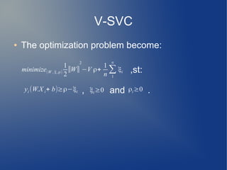
![Optimization Problem
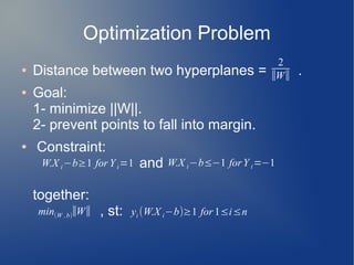
● Mathematically convenient:
, st:
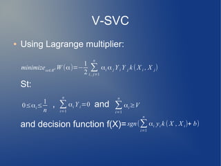
● By Lagrange multiplier , the problem become
quadratic optimization problem.
arg min(W ,b)
1
2
∣∣W∣∣
2
yi (W.X i−b)≥1
arg min(W ,b) max(α> 0)
1
2
∣∣W∣∣
2
−∑
i=1
n
αi [ yi (W.X i−b)−1]](https://image.slidesharecdn.com/svmv-svc-150930130845-lva1-app6891/85/Svm-V-SVC-18-320.jpg)
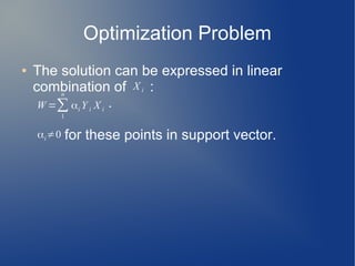


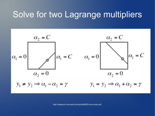
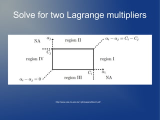
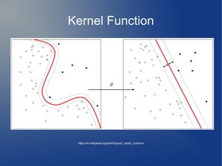
![Solve for two Lagrange multipliers
double X = Kii+Kjj+2*Kij;
double delta = (-G[i]-G[j])/X;
double diff = alpha[i] - alpha[j];
alpha[i] += delta; alpha[j] += delta;
if(region I):
alpha[i] = C_i; alpha[j] = C_i – diff;
if(region II):
alpha[j] = C_j; alpha[i] = C_j + diff;
if(region III):
alpha[j] = 0;alpha[i] = diff;
If (region IV):
alpha[i] = 0;alpha[j] = -diff;](https://image.slidesharecdn.com/svmv-svc-150930130845-lva1-app6891/85/Svm-V-SVC-35-320.jpg)
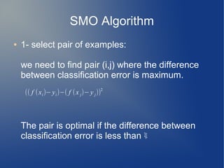
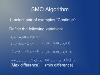
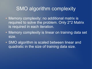

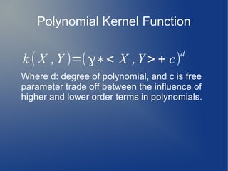
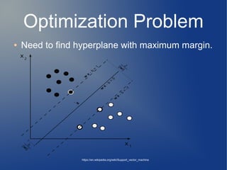
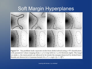
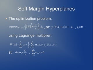
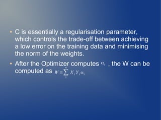
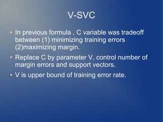
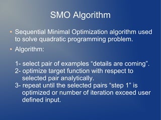
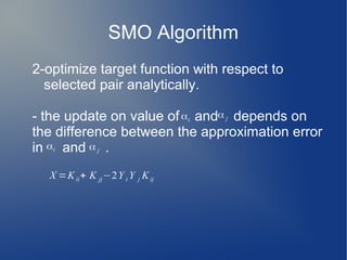
Support Vector Machine (SVM) is a supervised learning model used for classification and regression analysis. It finds the optimal separating hyperplane between classes that maximizes the margin between them. Kernel functions like polynomial, RBF, and sigmoid kernels allow SVMs to perform nonlinear classification by mapping inputs into high-dimensional feature spaces. The optimization problem of finding the hyperplane is solved using techniques like Lagrange multipliers and the Sequential Minimal Optimization (SMO) algorithm, which breaks the large QP problem into smaller subproblems solved analytically. SMO selects pairs of examples to update their Lagrange multipliers until convergence.