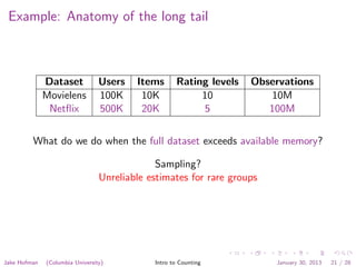
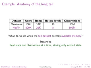
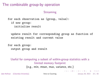
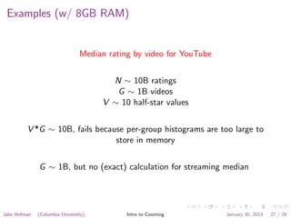
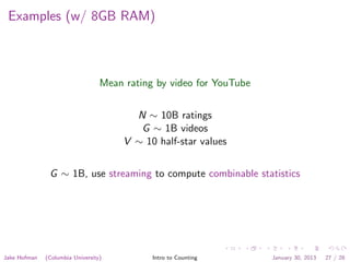
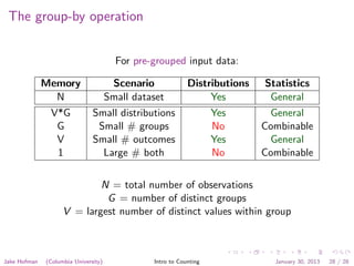
This document introduces counting and grouping large datasets. It discusses how to compute statistics on data when the full dataset exceeds memory capacity. It presents three approaches to grouping data: loading the full dataset into memory, streaming to process one observation at a time, and storing per-group histograms. The approaches vary in the types of statistics that can be computed based on the number of observations, groups, and distinct values within each group.


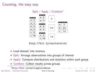


![Example: Movielens
0
1,000,000
2,000,000
3,000,000
1 2 3 4 5
Rating
Numberofratings
for each rating:
counts[movie id]++
Jake Hofman (Columbia University) Intro to Counting January 30, 2013 23 / 28](https://image.slidesharecdn.com/lecture2-150205203840-conversion-gate01/85/Modeling-Social-Data-Lecture-2-Introduction-to-Counting-35-320.jpg)
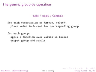
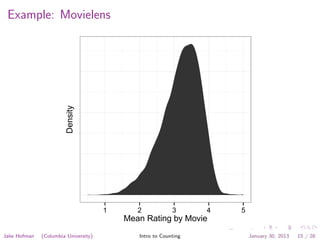
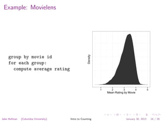
![Example: Movielens
for each rating:
totals[movie id] += rating
counts[movie id]++
for each group:
totals[movie id] /
counts[movie id]
1 2 3 4 5
Mean Rating by Movie
Density
Jake Hofman (Columbia University) Intro to Counting January 30, 2013 24 / 28](https://image.slidesharecdn.com/lecture2-150205203840-conversion-gate01/85/Modeling-Social-Data-Lecture-2-Introduction-to-Counting-36-320.jpg)
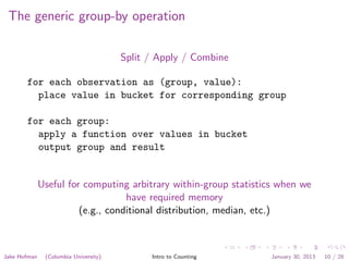
![Yet another group-by operation
Per-group histograms
for each observation as (group, value):
histogram[group][value]++
for each group:
compute result as a function of histogram
output group and result
Jake Hofman (Columbia University) Intro to Counting January 30, 2013 25 / 28](https://image.slidesharecdn.com/lecture2-150205203840-conversion-gate01/85/Modeling-Social-Data-Lecture-2-Introduction-to-Counting-37-320.jpg)
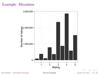
![Yet another group-by operation
Per-group histograms
for each observation as (group, value):
histogram[group][value]++
for each group:
compute result as a function of histogram
output group and result
We can recover arbitrary statistics if we can afford to store counts
of all distinct values within in each group
Jake Hofman (Columbia University) Intro to Counting January 30, 2013 25 / 28](https://image.slidesharecdn.com/lecture2-150205203840-conversion-gate01/85/Modeling-Social-Data-Lecture-2-Introduction-to-Counting-38-320.jpg)


![[RIIT 2017] Identifying Grey Sheep Users By The Distribution of User Similari...](https://cdn.slidesharecdn.com/ss_thumbnails/slidegsuser-171004030338-thumbnail.jpg?width=640&height=640&fit=bounds)
![[WI 2017] Context Suggestion: Empirical Evaluations vs User Studies](https://cdn.slidesharecdn.com/ss_thumbnails/slidewicontextsuggestion-170812014320-thumbnail.jpg?width=640&height=640&fit=bounds)


