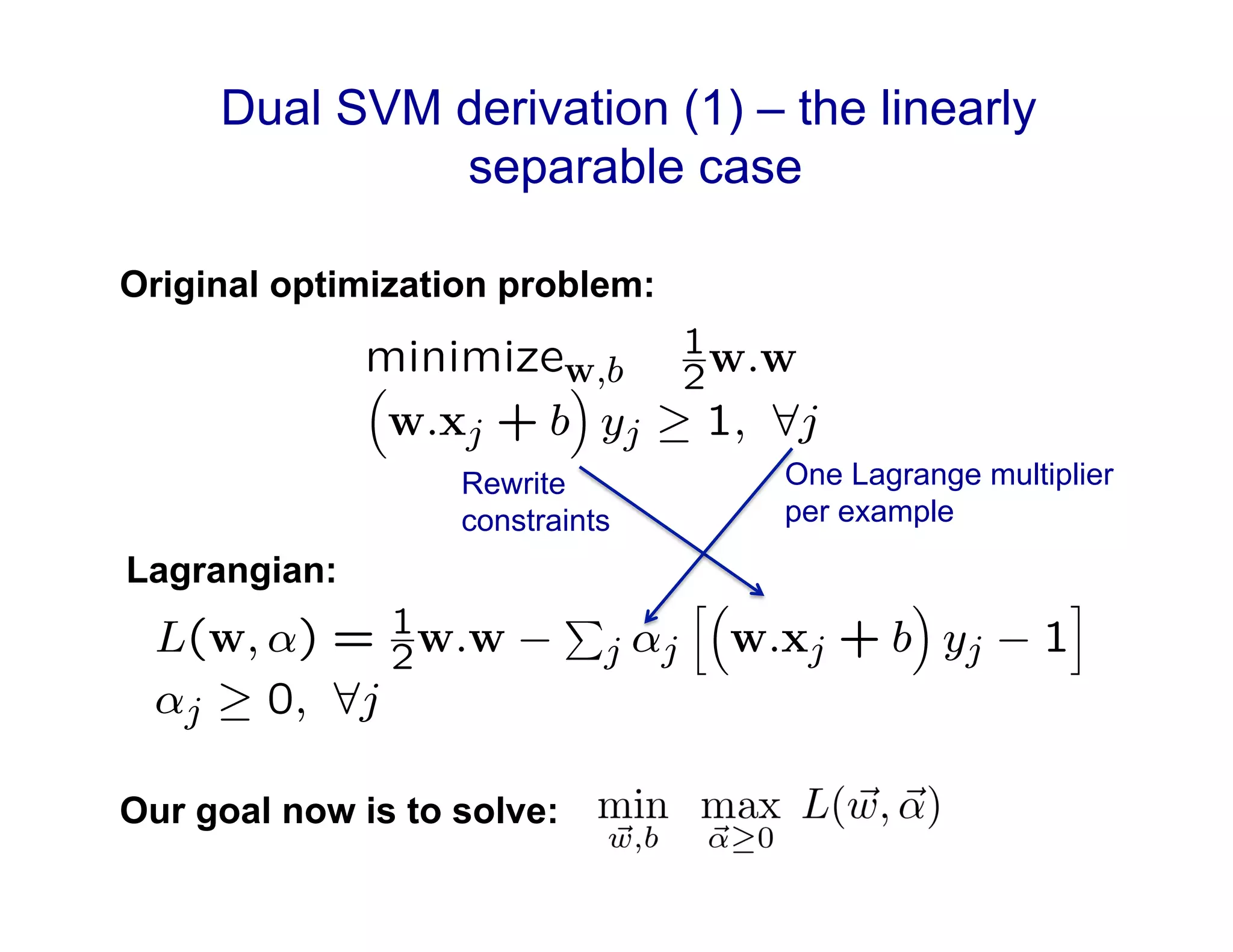
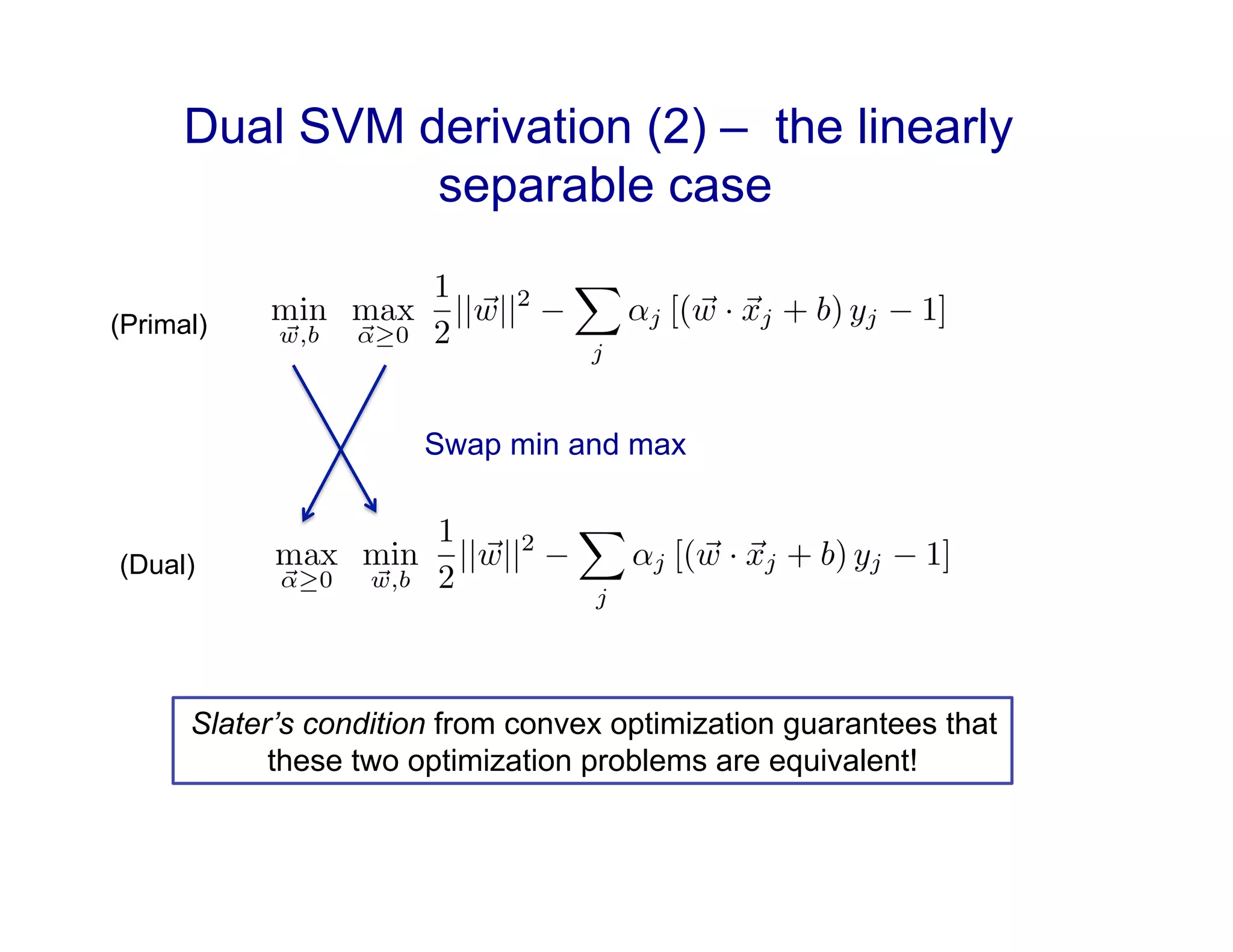
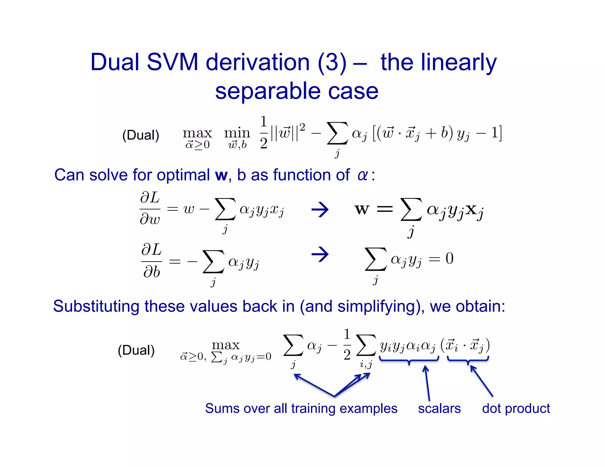
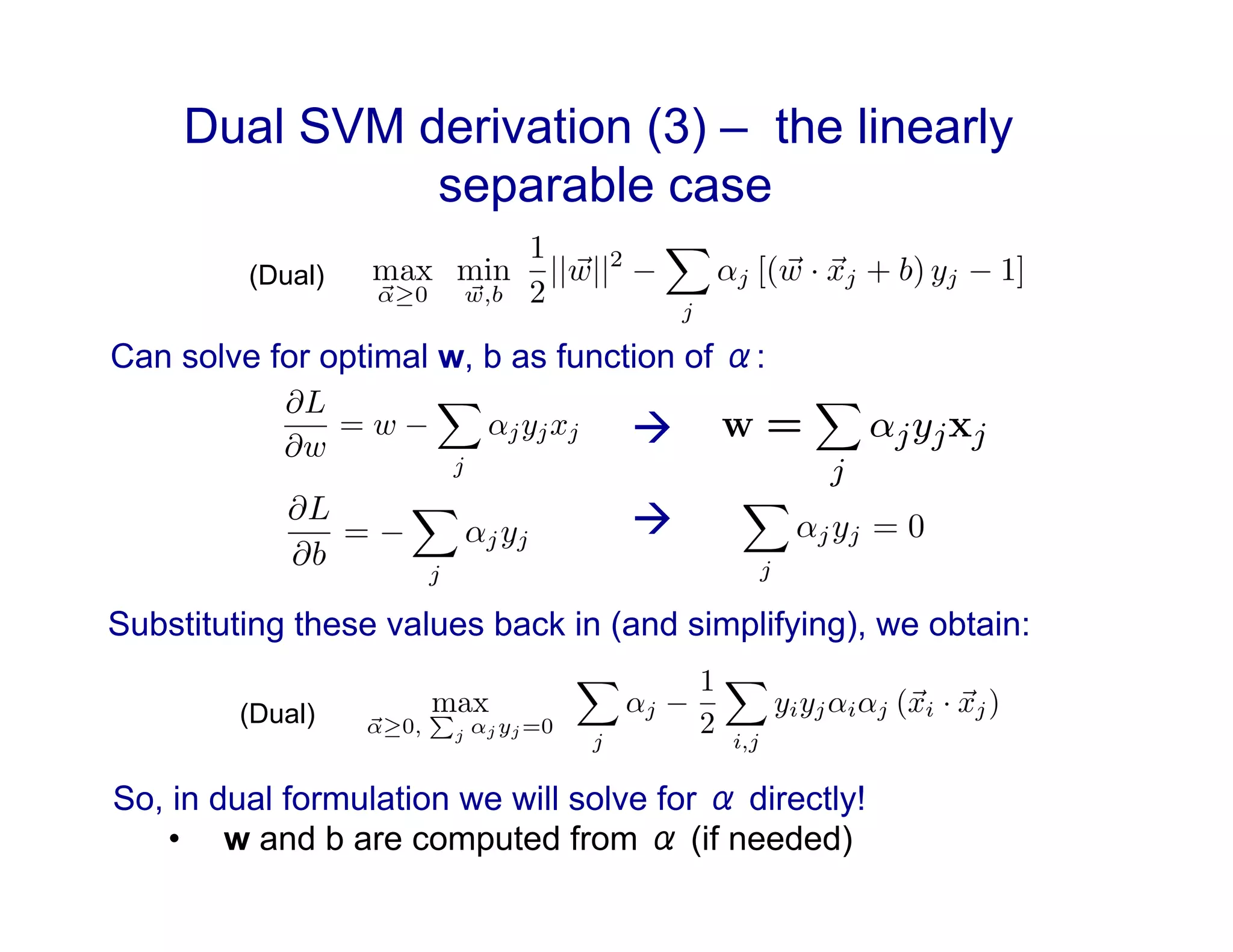
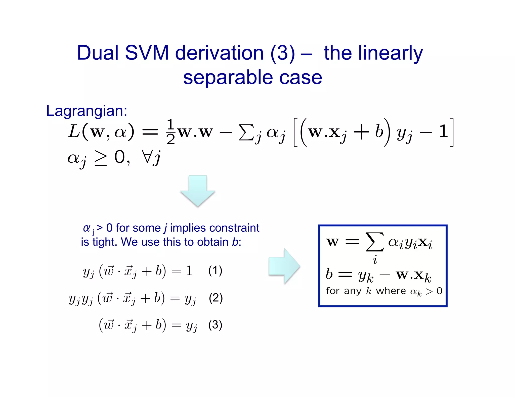
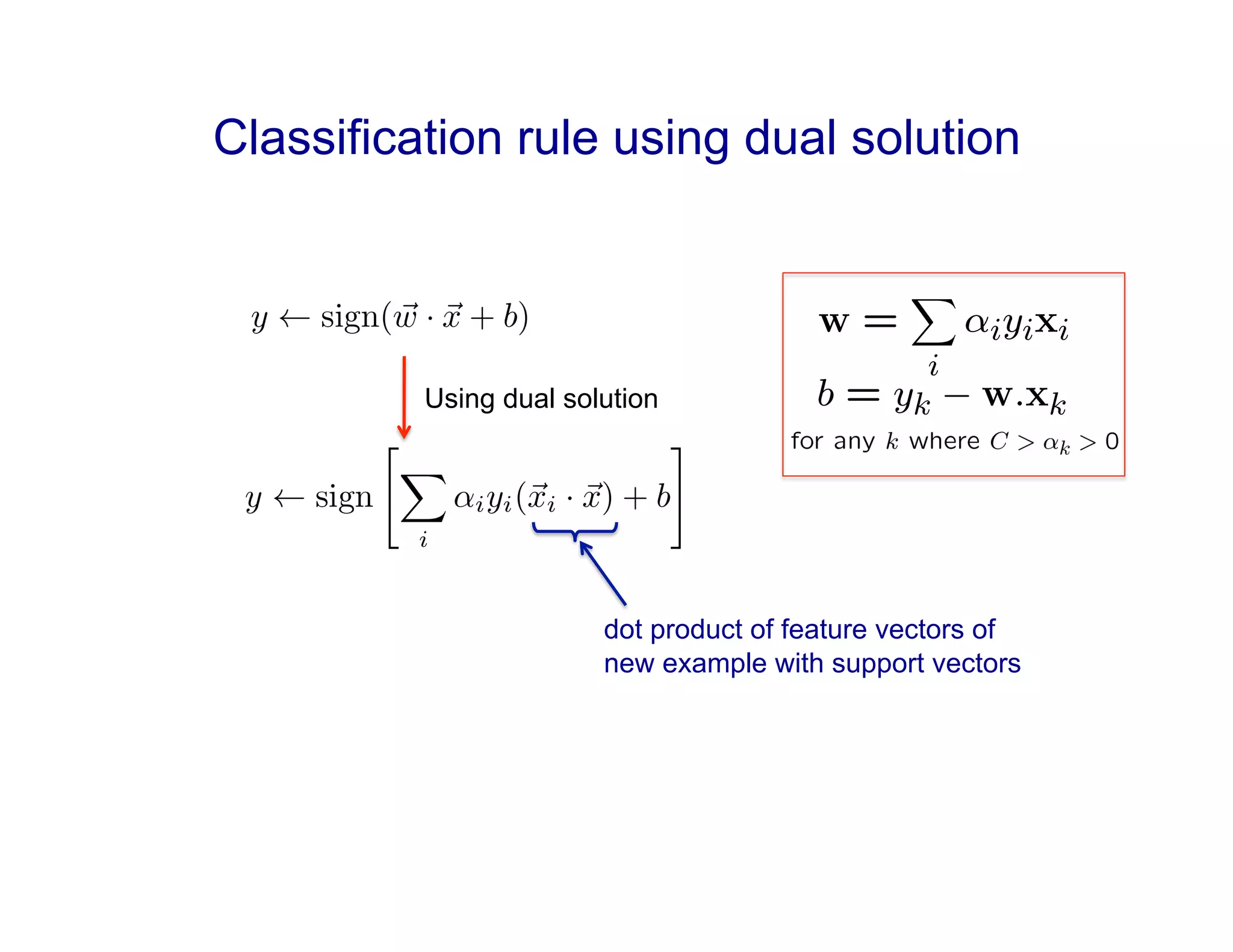
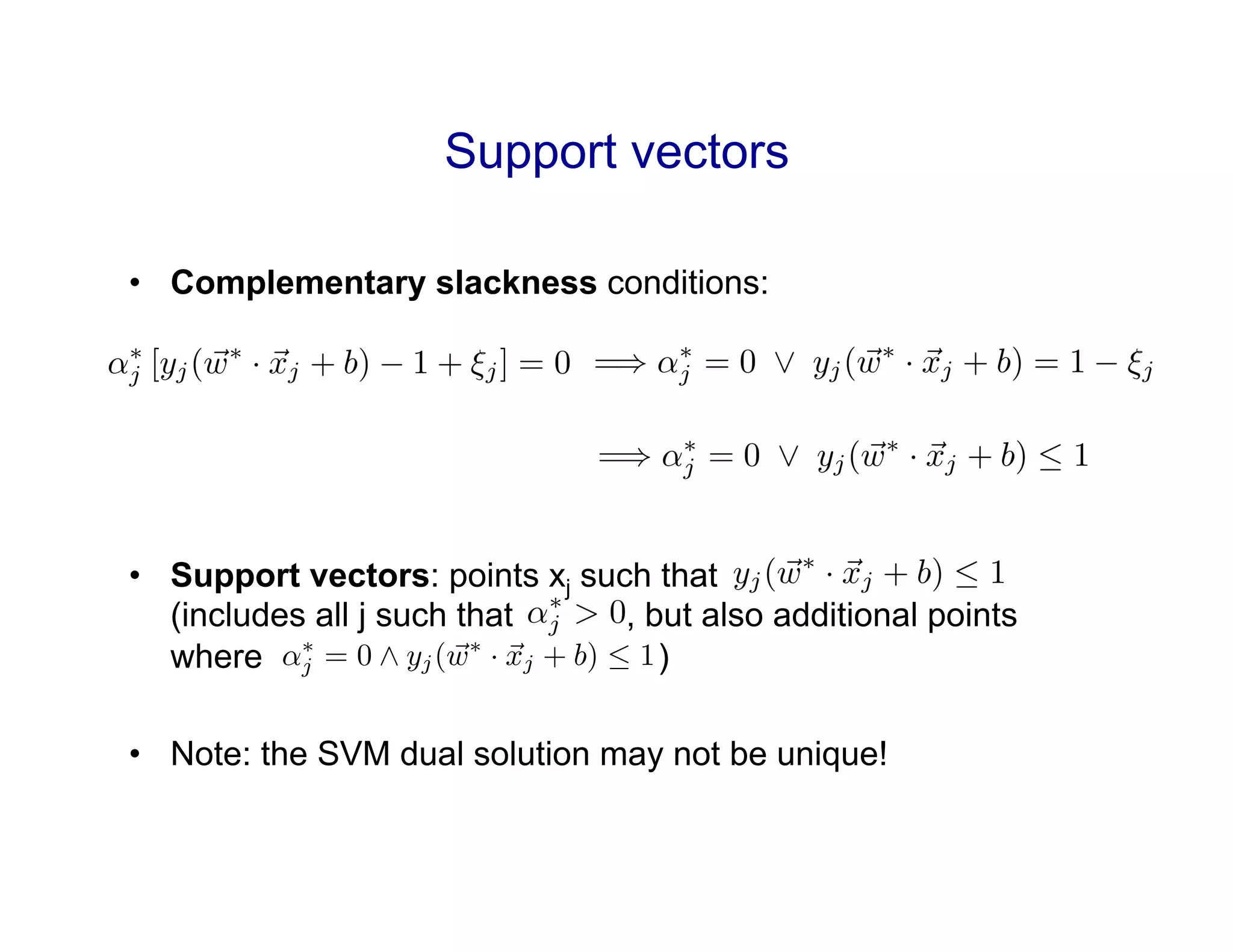
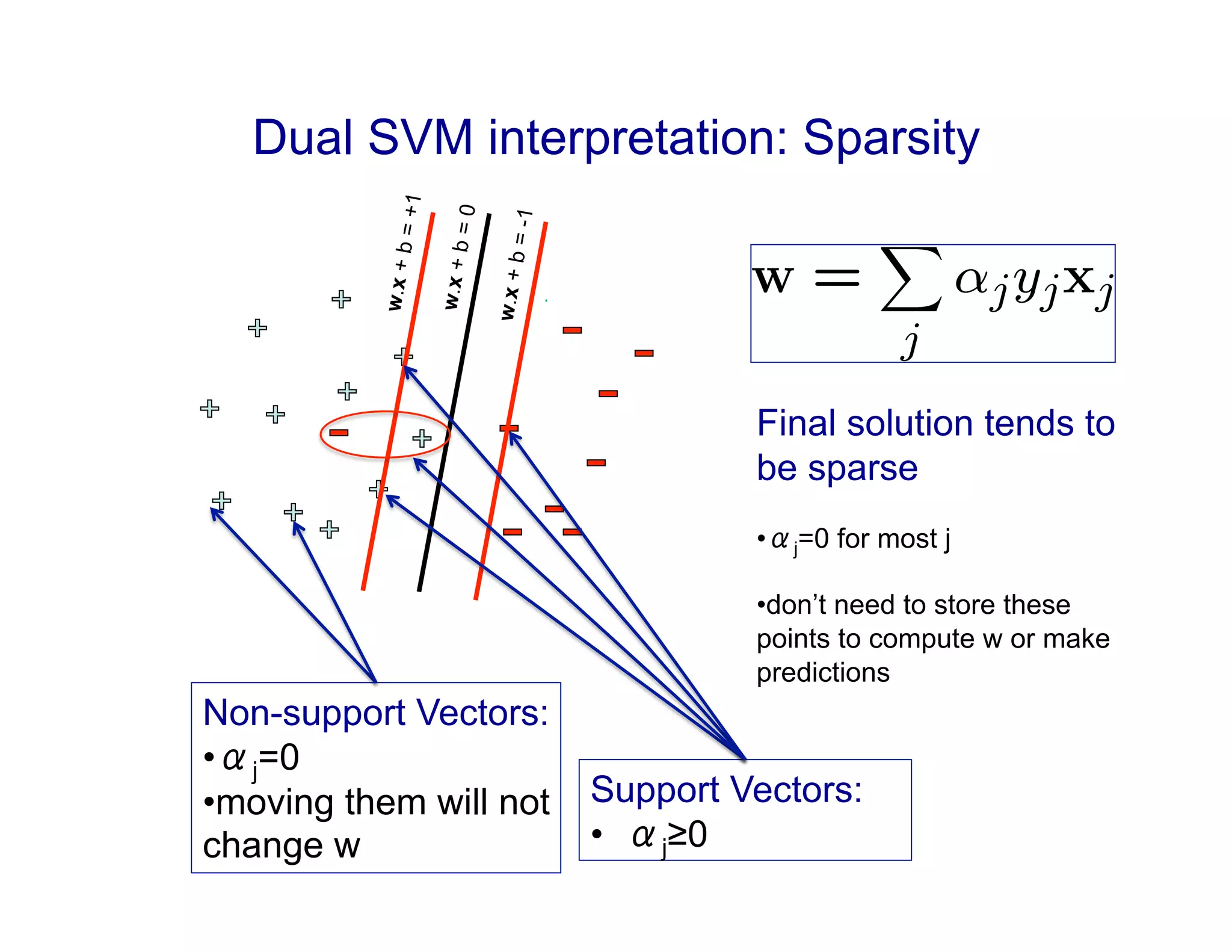
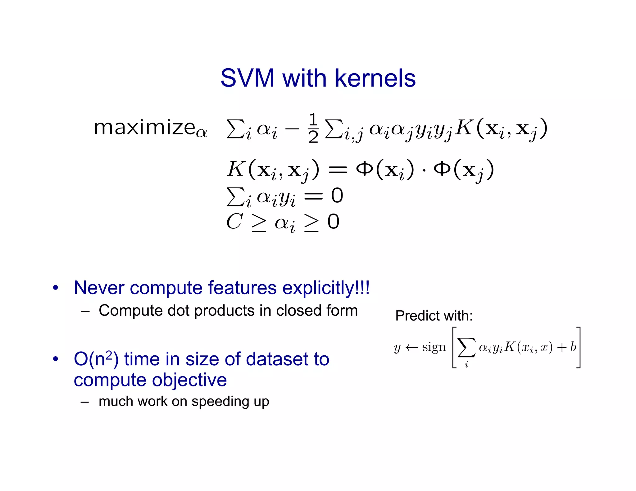
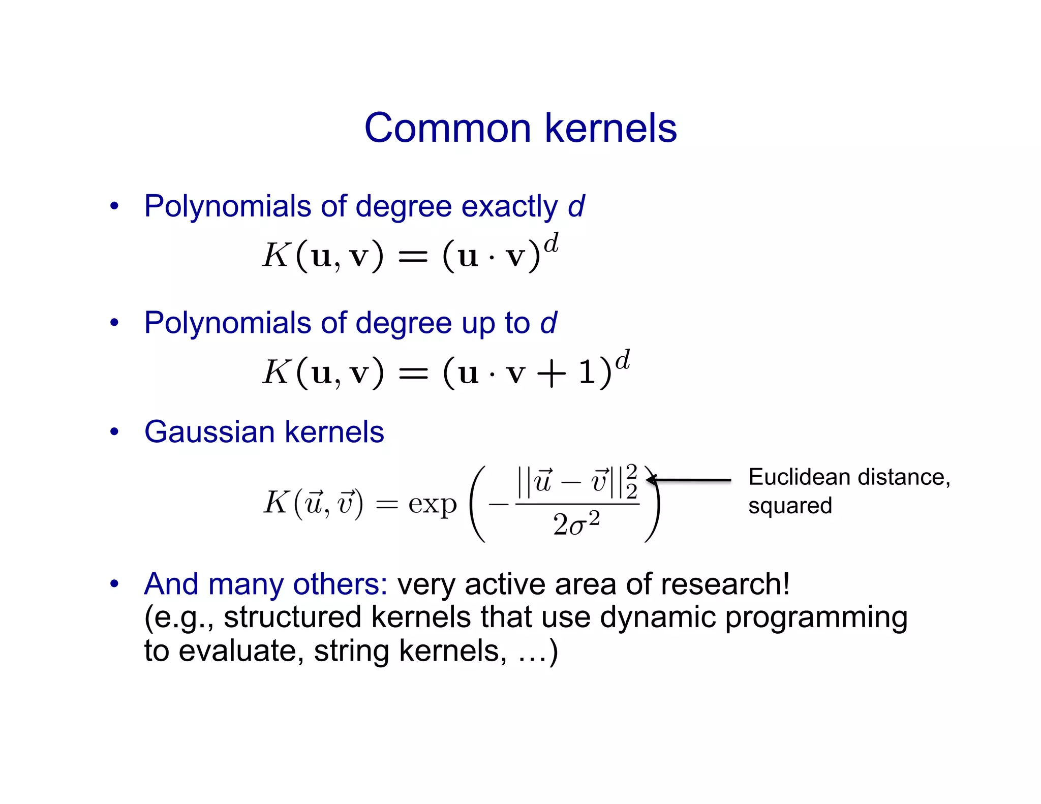
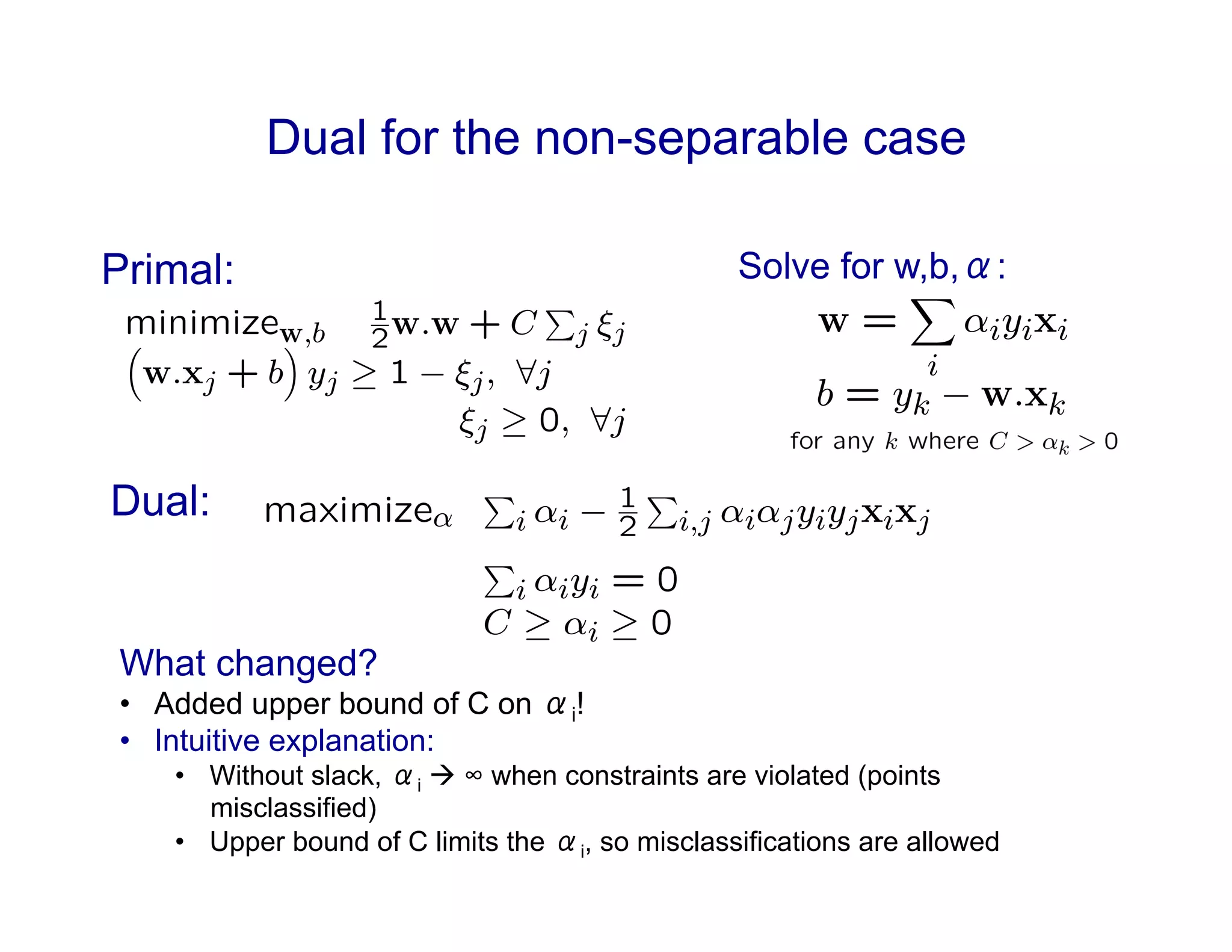
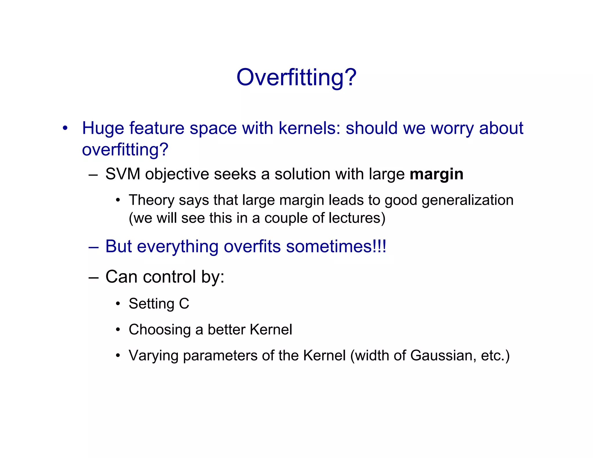
1) The document discusses support vector machines and kernels. It covers the derivation of the dual formulation of SVMs, which allows solving directly for the α values rather than w and b. 2) It explains how kernels can be used to transform data into a higher dimensional feature space without explicitly computing the features. Common kernels discussed include polynomial and Gaussian kernels. 3) The document notes that while kernels create a huge feature space, SVMs seek a large margin solution to generalize well, but overfitting can still occur and needs to be controlled through parameters like C and the kernel.

1. Support Vector Machines & Kernels
Lecture 6
David Sontag
New York University
Slides adapted from Luke Zettlemoyer and Carlos Guestrin,
and Vibhav Gogate

2. Dual SVM derivation (1) – the linearly
separable case
Original optimization problem:
Lagrangian:
Rewrite
constraints
One Lagrange multiplier
per example
Our goal now is to solve:

3. Dual SVM derivation (2) – the linearly
separable case
Swap min and max
Slater’s condition from convex optimization guarantees that
these two optimization problems are equivalent!
(Primal)
(Dual)

4. Dual SVM derivation (3) – the linearly
separable case
Can solve for optimal w, b as function of α:

⇥(x) =
⇧
⇧
⇧
⇧
⇧
⇧
⇧
⇧
⇧
⇧
⇧
⇤
x(1)
. . .
x(n)
x(1)x(2)
x(1)x(3)
. . .
ex(1)
. . .
⇥
⌃
⌃
⌃
⌃
⌃
⌃
⌃
⌃
⌃
⌃
⌃
⌅
⇤L
⇤w
= w
⌥
j
jyjxj
(Dual)

Substituting these values back in (and simplifying), we obtain:
(Dual)
Sums over all training examples dot product
scalars

5. Dual SVM derivation (3) – the linearly
separable case
Can solve for optimal w, b as function of α:

⇥(x) =
⇧
⇧
⇧
⇧
⇧
⇧
⇧
⇧
⇧
⇧
⇧
⇤
x(1)
. . .
x(n)
x(1)x(2)
x(1)x(3)
. . .
ex(1)
. . .
⇥
⌃
⌃
⌃
⌃
⌃
⌃
⌃
⌃
⌃
⌃
⌃
⌅
⇤L
⇤w
= w
⌥
j
jyjxj
So, in dual formulation we will solve for α directly!
• w and b are computed from α (if needed)
(Dual)

Substituting these values back in (and simplifying), we obtain:
(Dual)

6. Dual SVM derivation (3) – the linearly
separable case
Lagrangian:
αj > 0 for some j implies constraint
is tight. We use this to obtain b:
(1)
(2)
(3)

7. Classification rule using dual solution
Using dual solution
dot product of feature vectors of
new example with support vectors

8. Dual for the non-separable case
Primal: Solve for w,b,α:
Dual:
What changed?
• Added upper bound of C on αi!
• Intuitive explanation:
• Without slack, αi  ∞ when constraints are violated (points
misclassified)
• Upper bound of C limits the αi, so misclassifications are allowed

9. Support vectors
• Complementary slackness conditions:
• Support vectors: points xj such that
(includes all j such that , but also additional points
where )
• Note: the SVM dual solution may not be unique!
↵⇤
j = 0 ^ yj(~
w⇤
· ~
xj + b)  1

10. Dual SVM interpretation: Sparsity
w
.
x
+
b
=
+
1
w
.
x
+
b
=
-
1
w
.
x
+
b
=
0
Support Vectors:
• αj≥0
Non-support Vectors:
• αj=0
• moving them will not
change w
Final solution tends to
be sparse
• αj=0 for most j
• don’t need to store these
points to compute w or make
predictions

11. SVM with kernels
• Never compute features explicitly!!!
– Compute dot products in closed form
• O(n2) time in size of dataset to
compute objective
– much work on speeding up
Predict with:

12. [Tommi Jaakkola]
Quadratic kernel

13. Quadratic kernel
[Cynthia Rudin]
Feature mapping given by:

14. Common kernels
• Polynomials of degree exactly d
• Polynomials of degree up to d
• Gaussian kernels
• And many others: very active area of research!
(e.g., structured kernels that use dynamic programming
to evaluate, string kernels, …)
Euclidean distance,
squared

15. Gaussian kernel
[Cynthia Rudin] [mblondel.org]
Support vectors
Level sets, i.e. w.x=r for some r

16. Kernel algebra
[Justin Domke]
Q: How would you prove that the “Gaussian kernel” is a valid kernel?
A: Expand the Euclidean norm as follows:
Then, apply (e) from above
To see that this is a kernel, use the
Taylor series expansion of the
exponential, together with repeated
application of (a), (b), and (c):
The feature mapping is
infinite dimensional!

17. Overfitting?
• Huge feature space with kernels: should we worry about
overfitting?
– SVM objective seeks a solution with large margin
• Theory says that large margin leads to good generalization
(we will see this in a couple of lectures)
– But everything overfits sometimes!!!
– Can control by:
• Setting C
• Choosing a better Kernel
• Varying parameters of the Kernel (width of Gaussian, etc.)