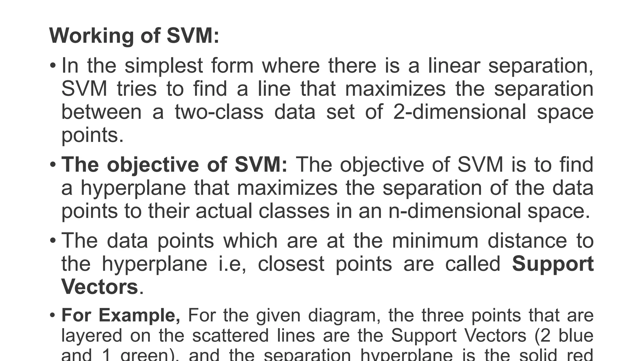
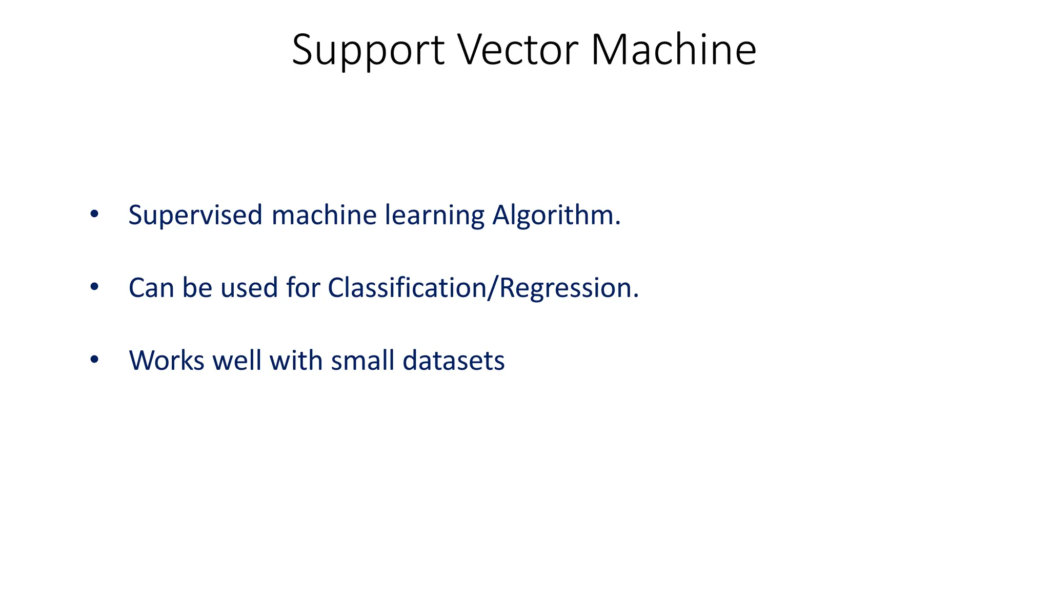
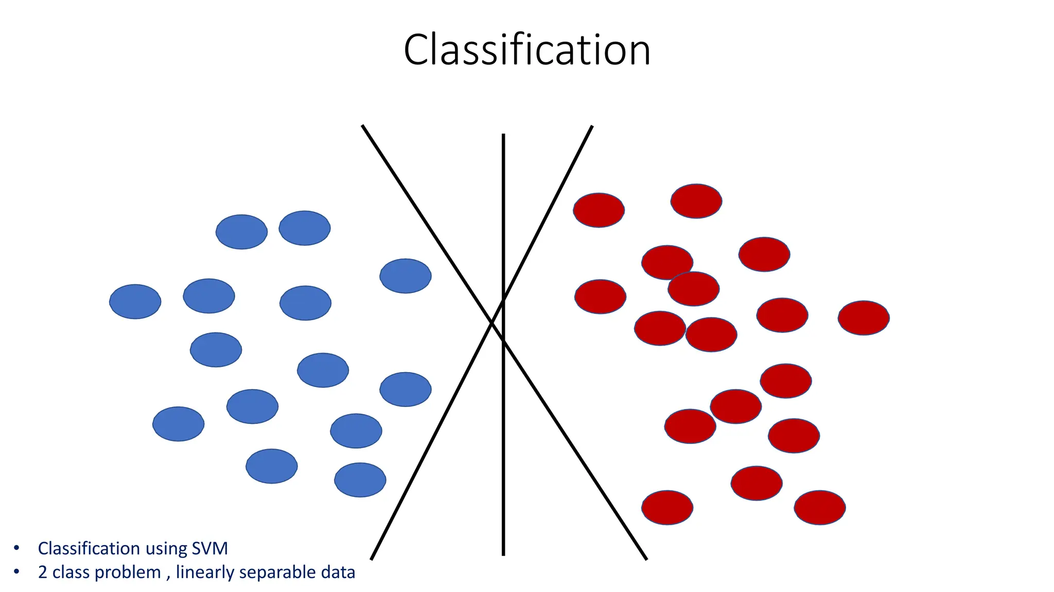
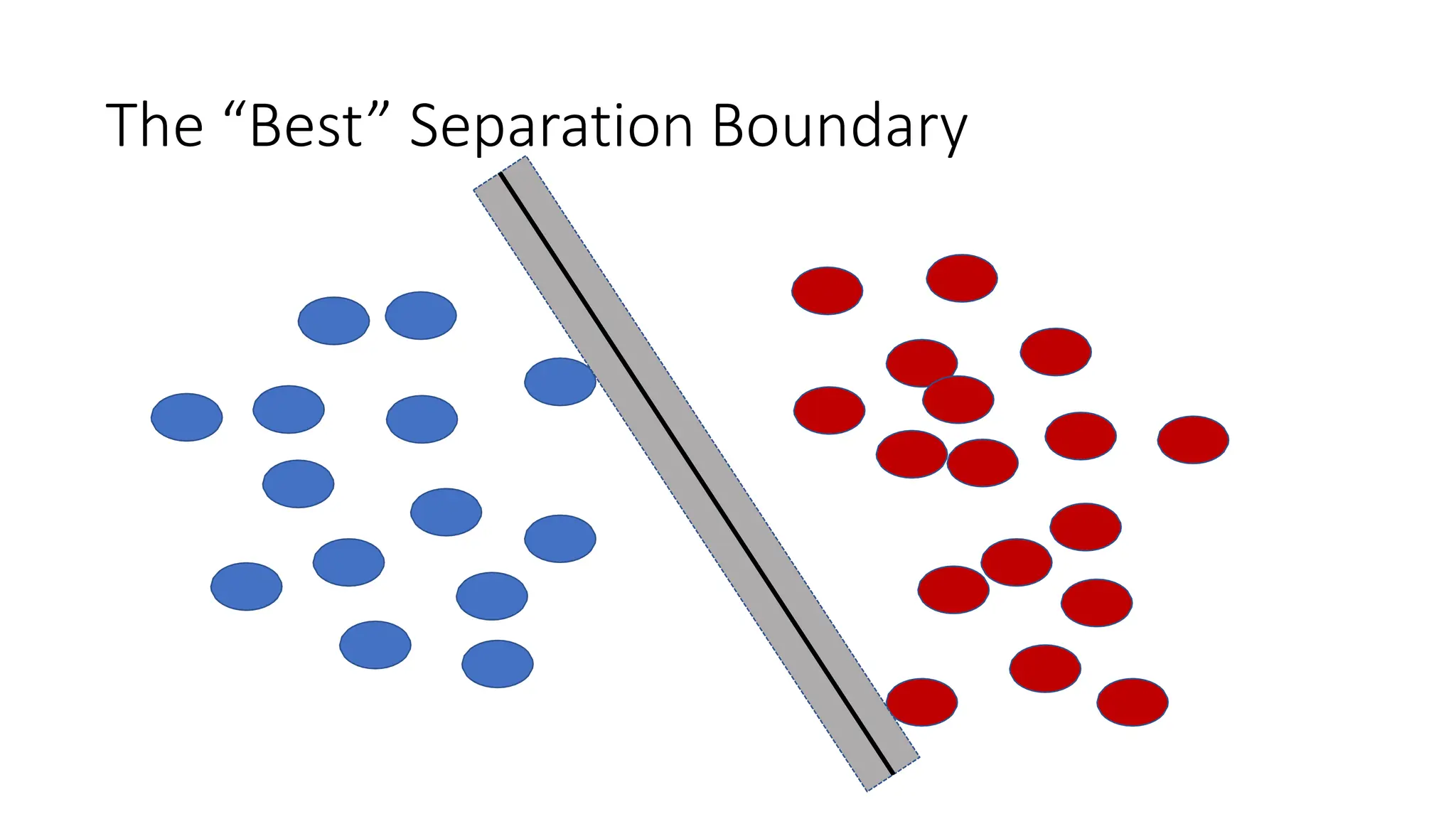
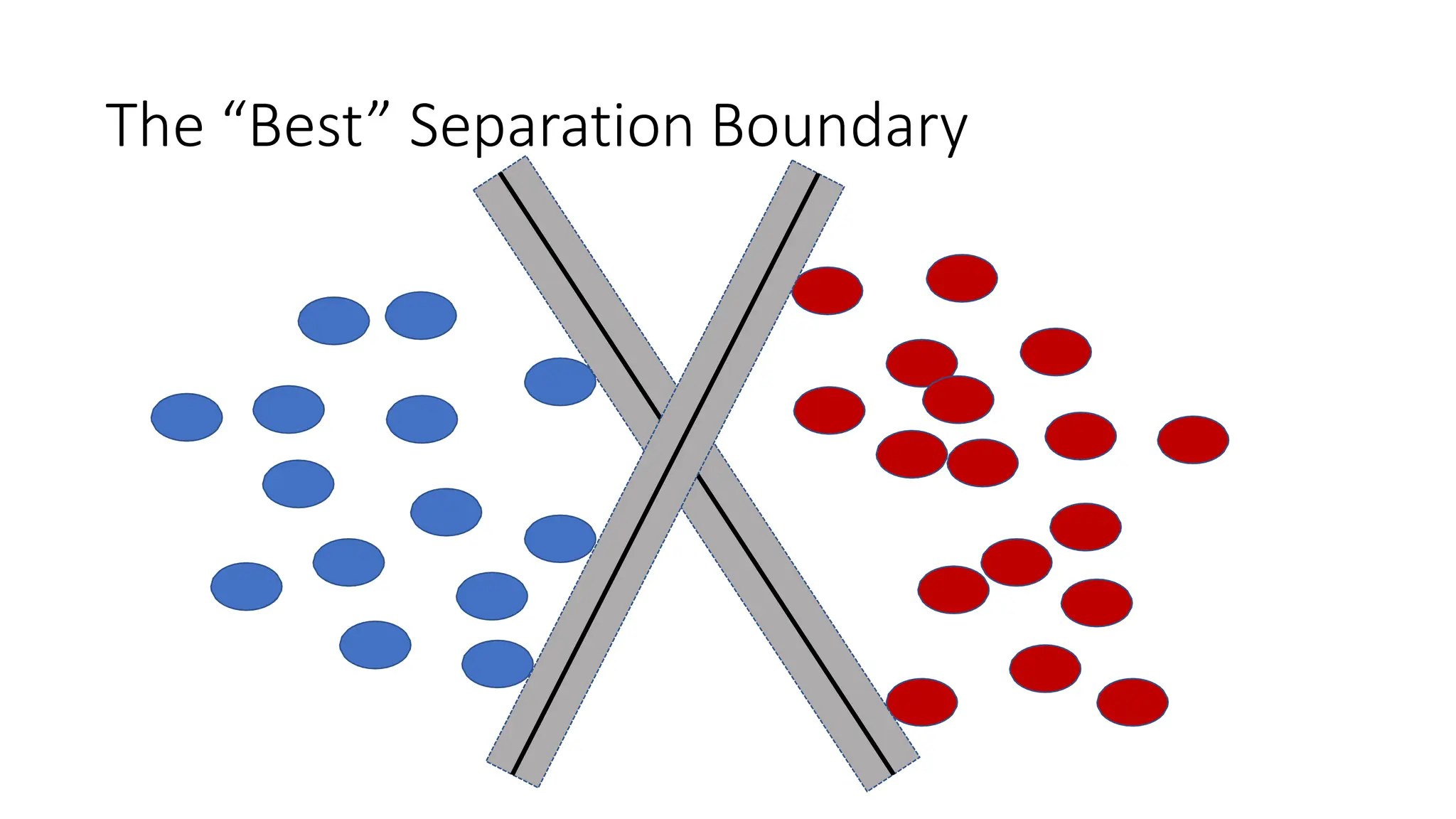
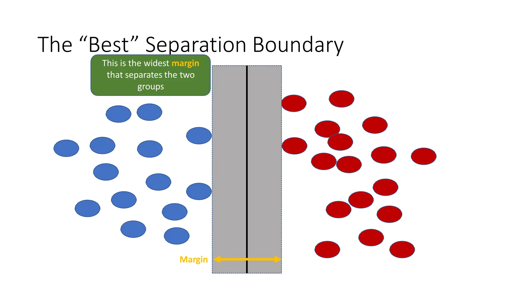
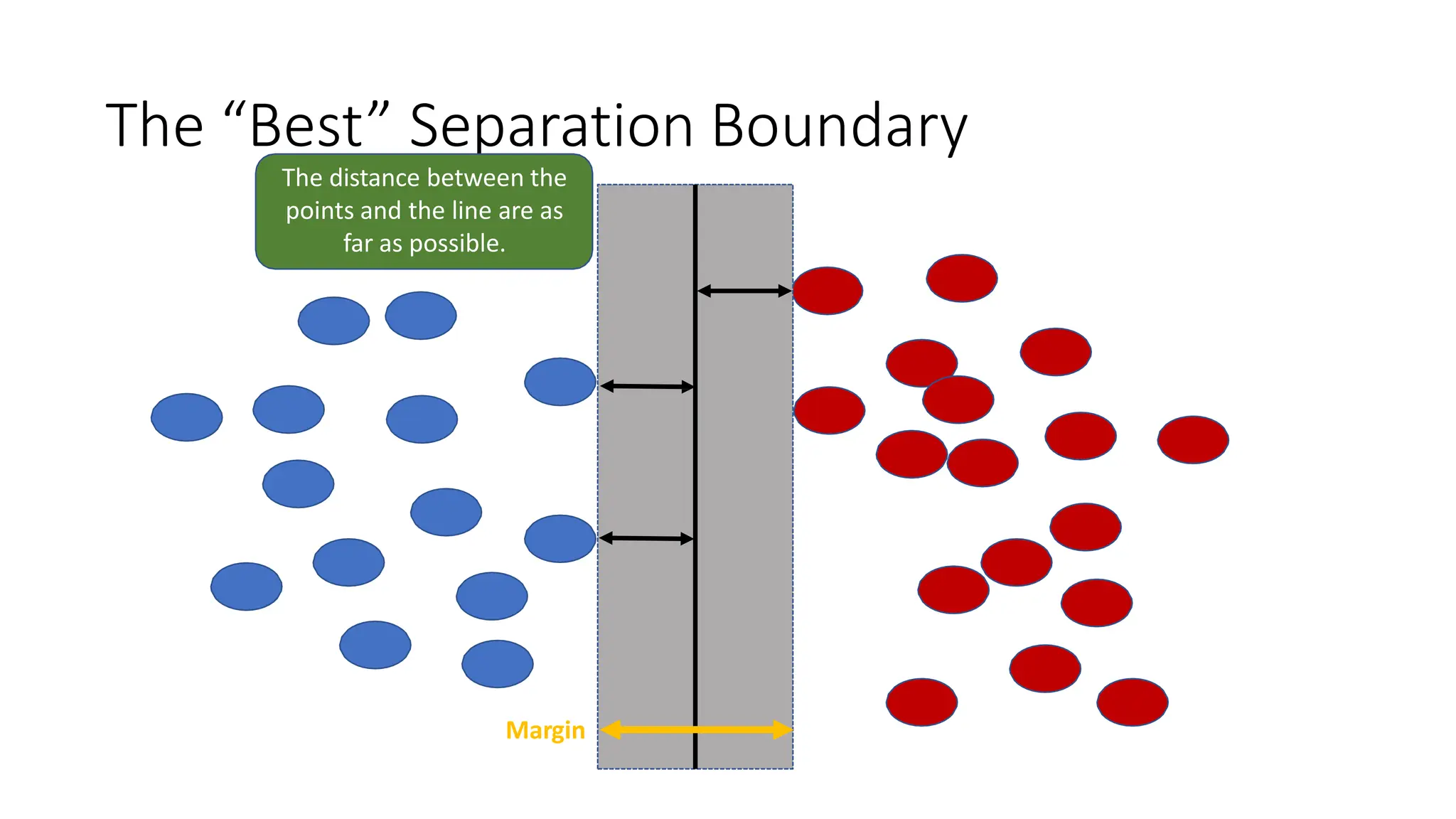
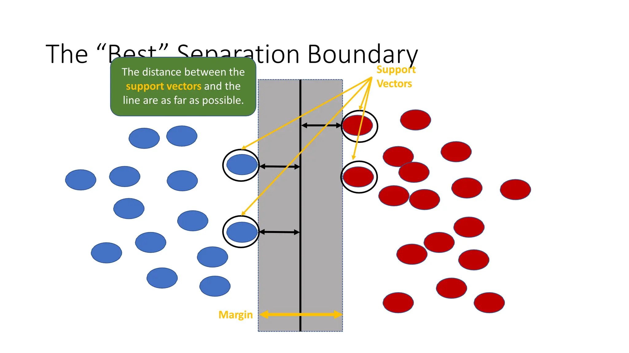
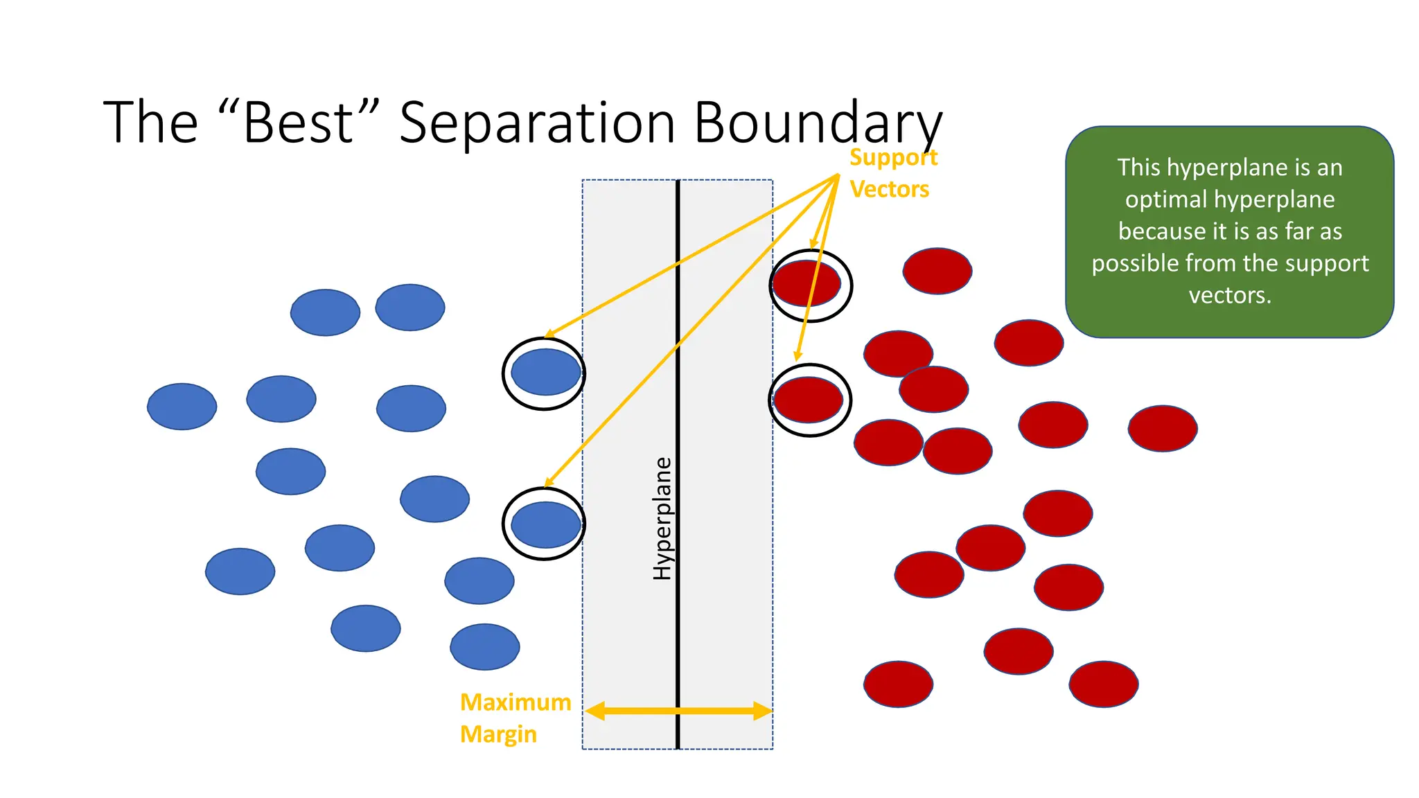
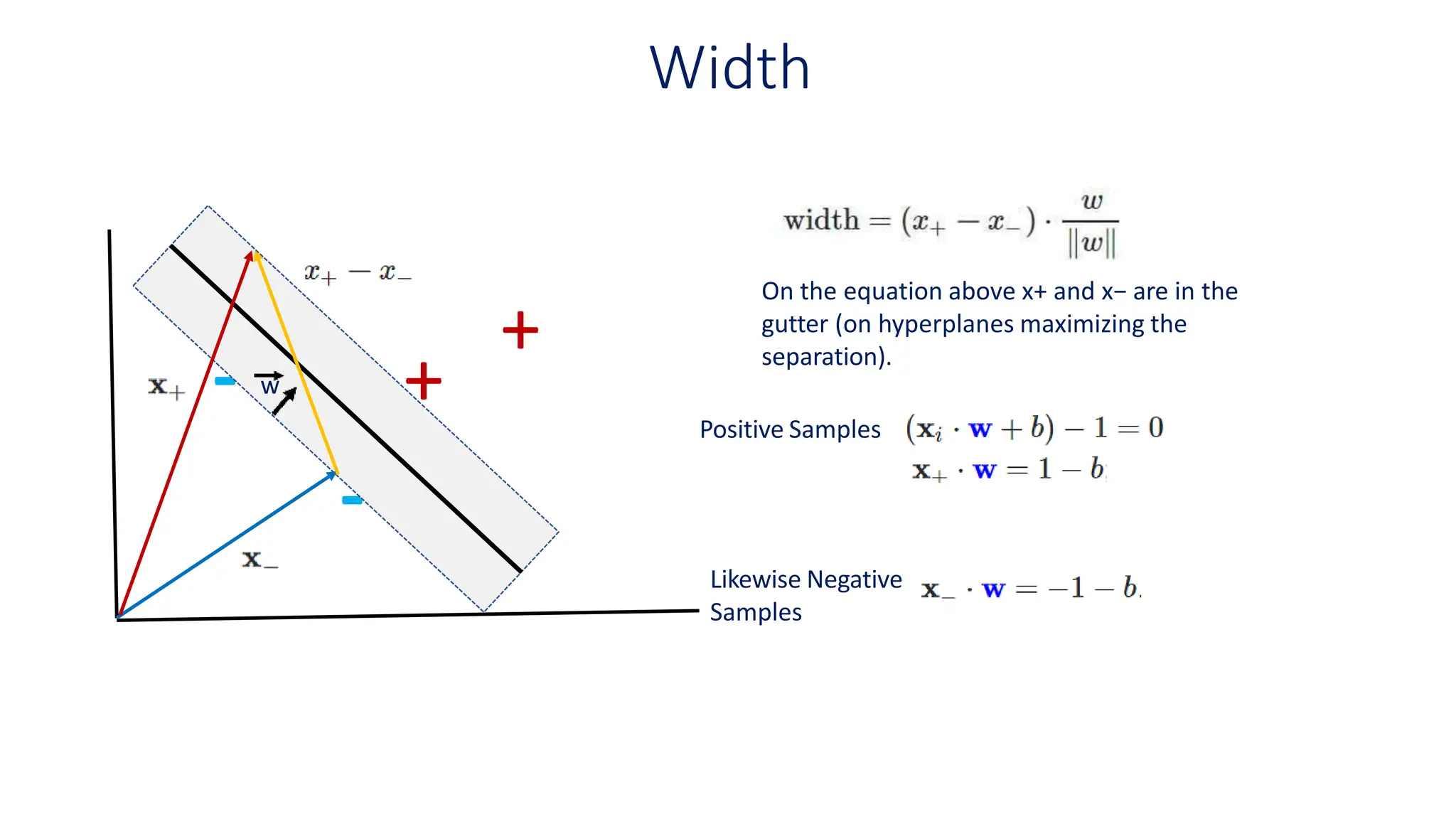
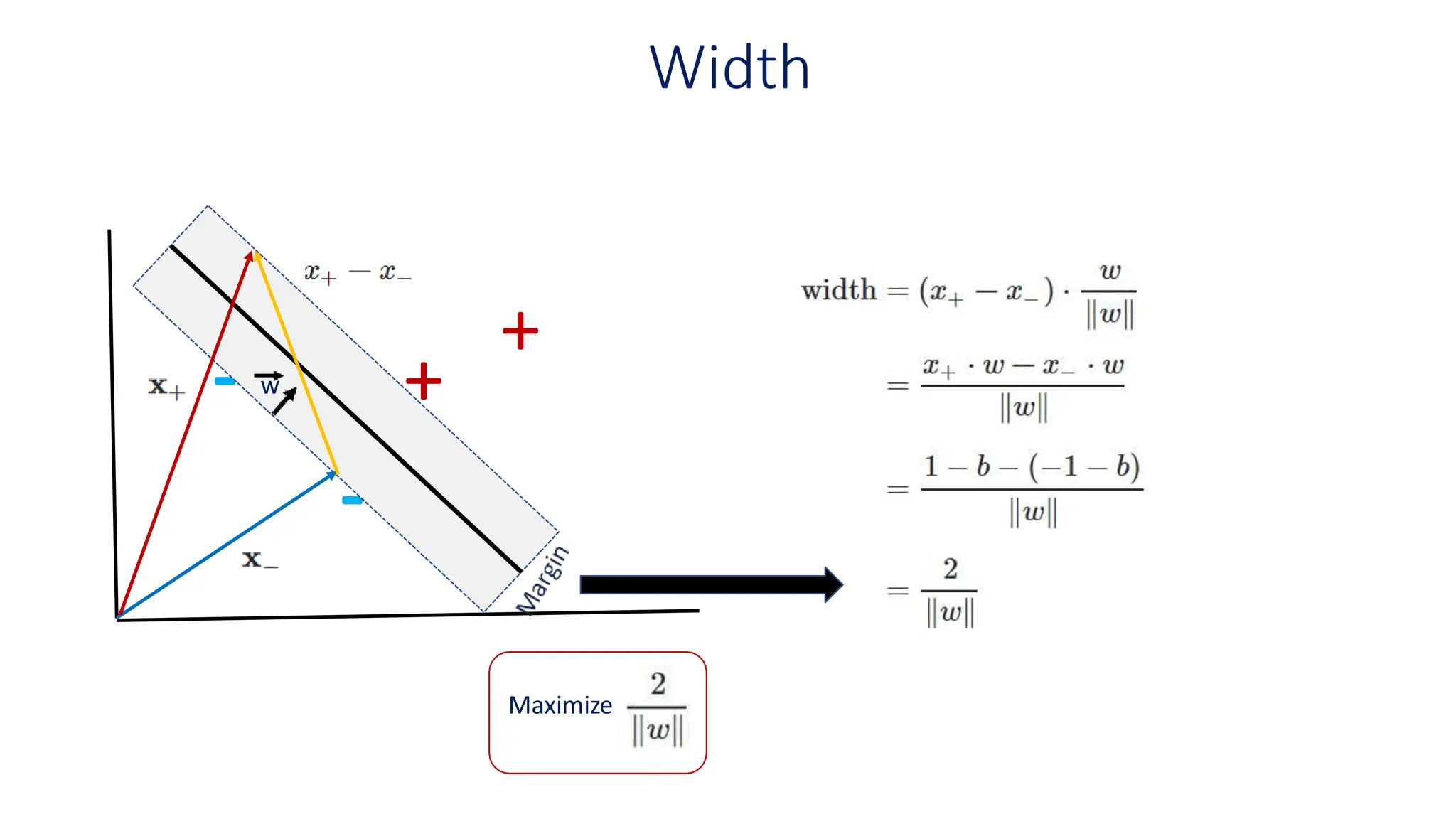
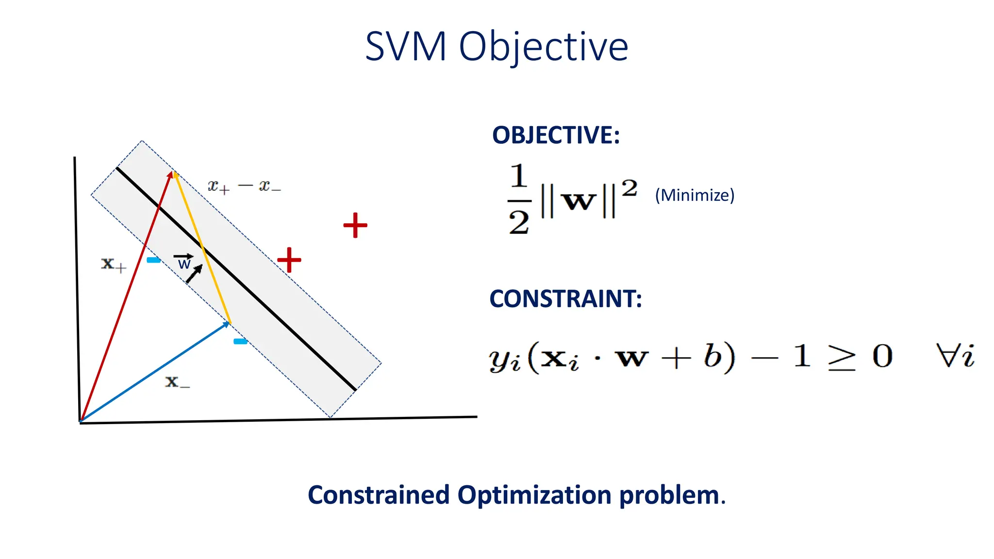
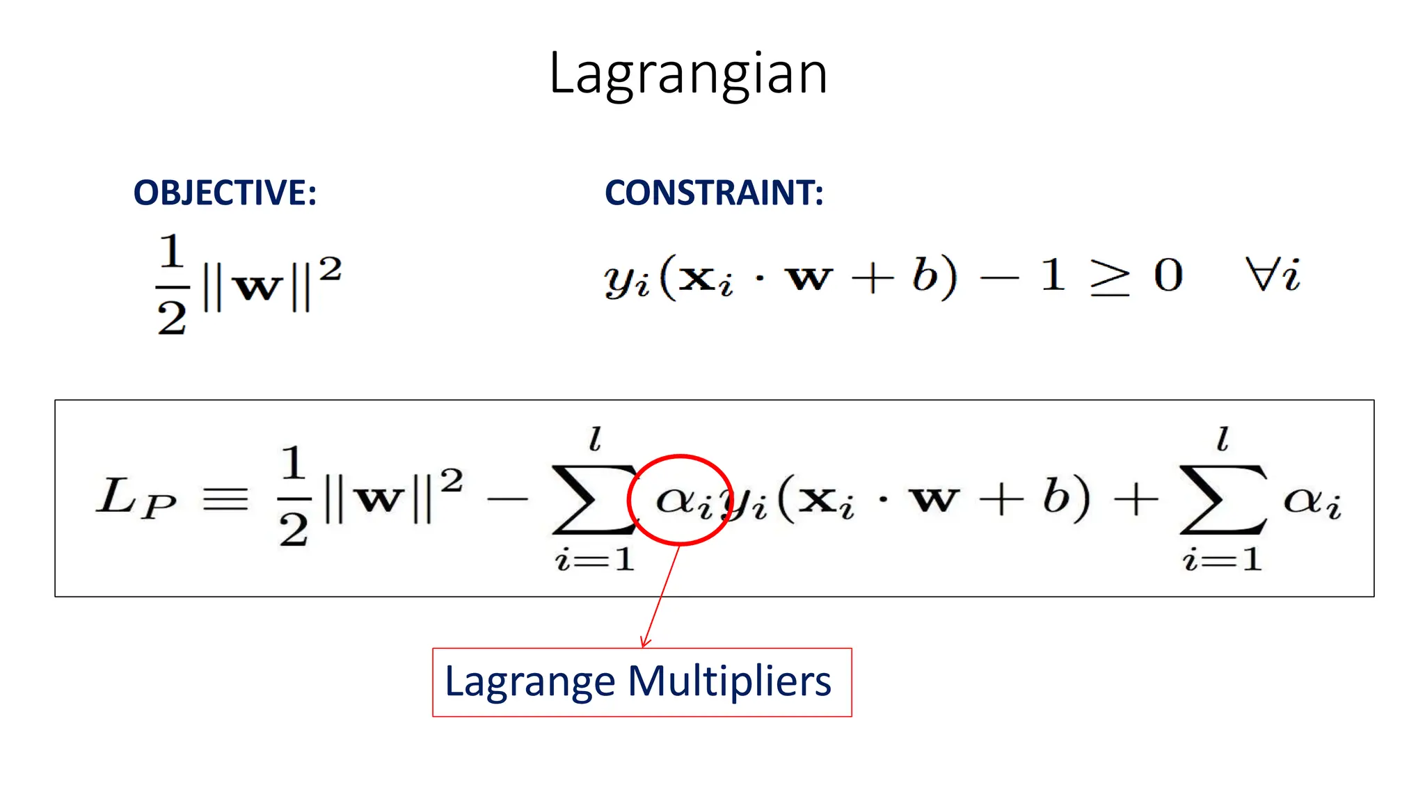
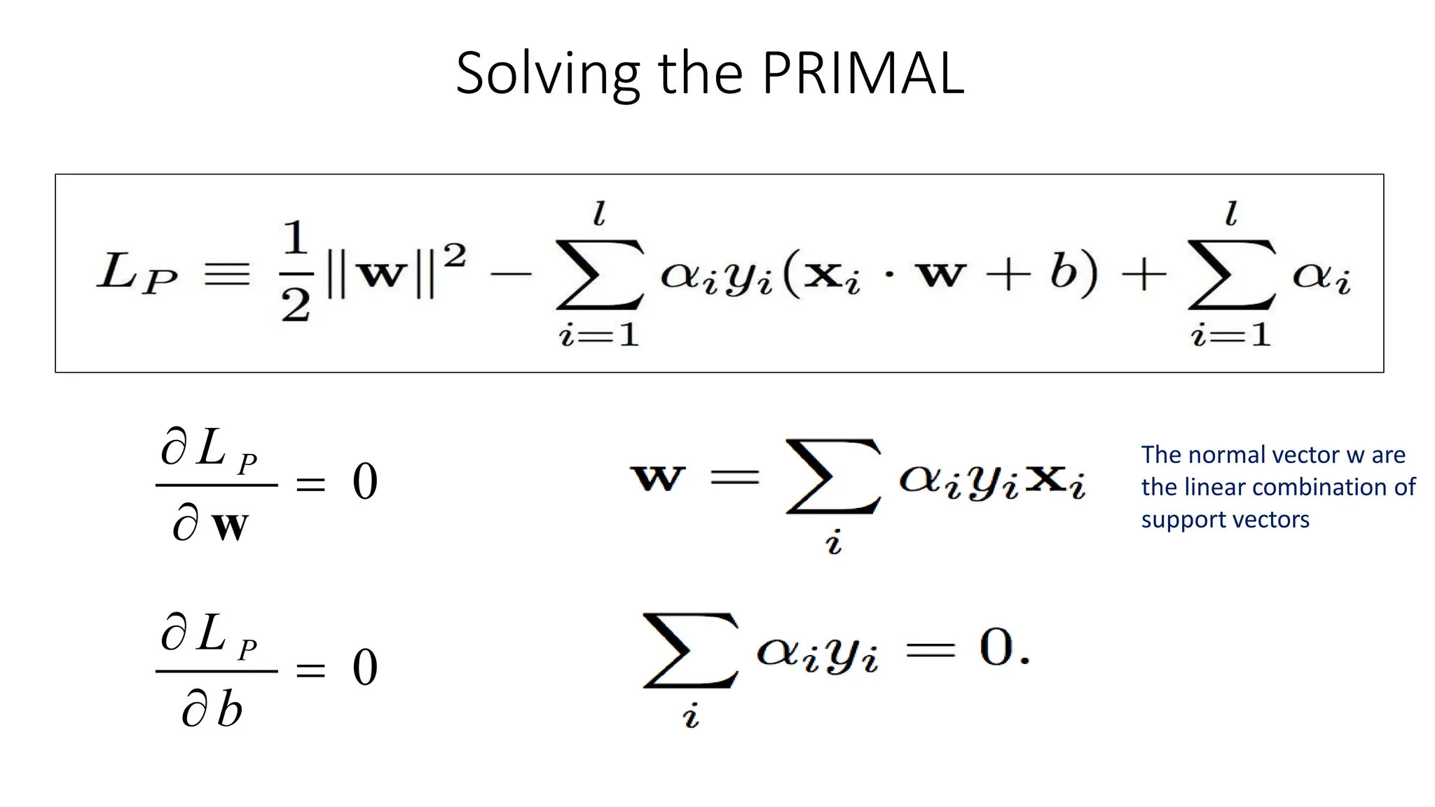
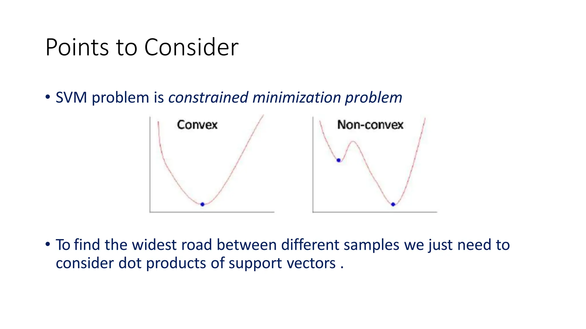
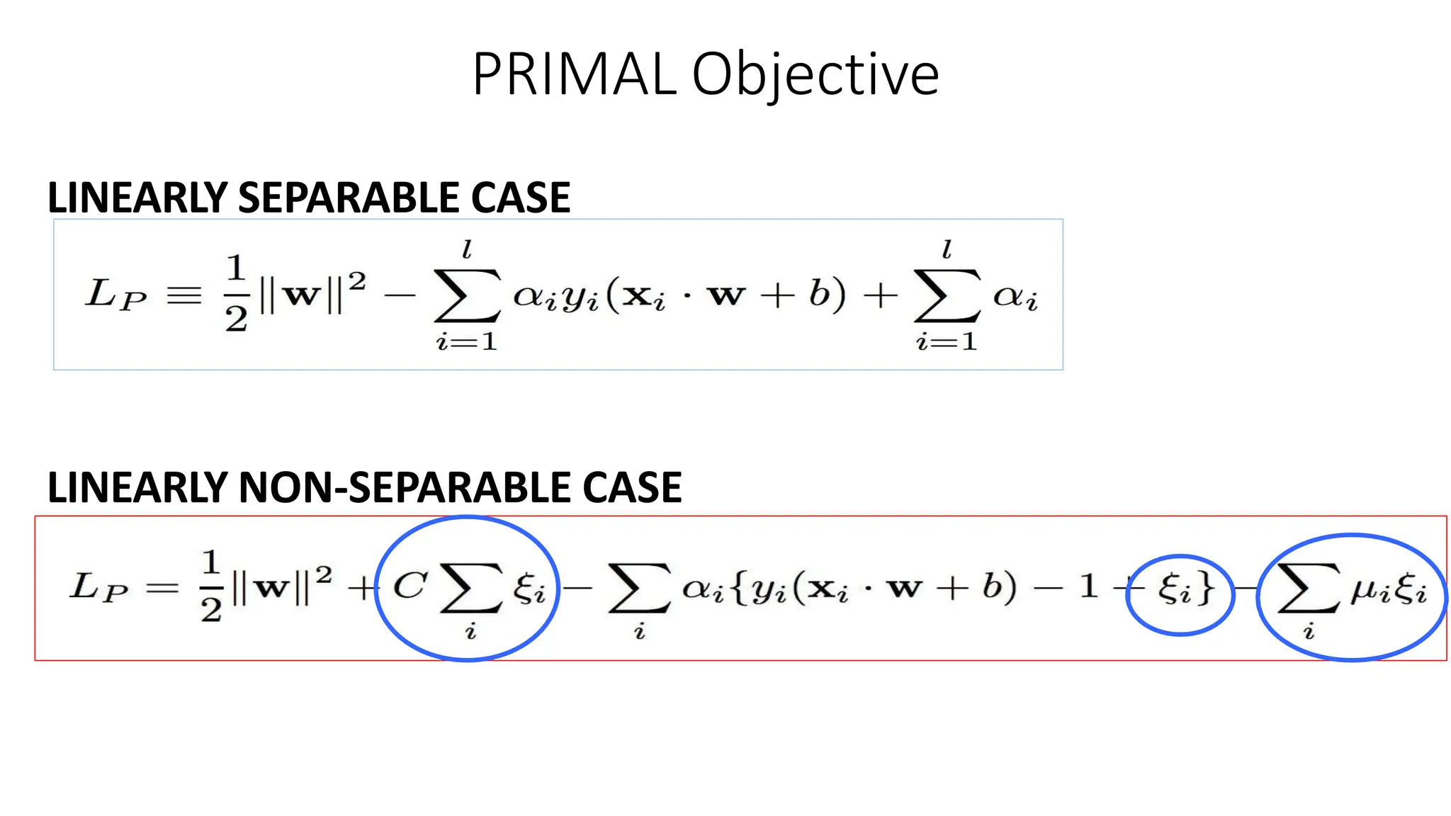
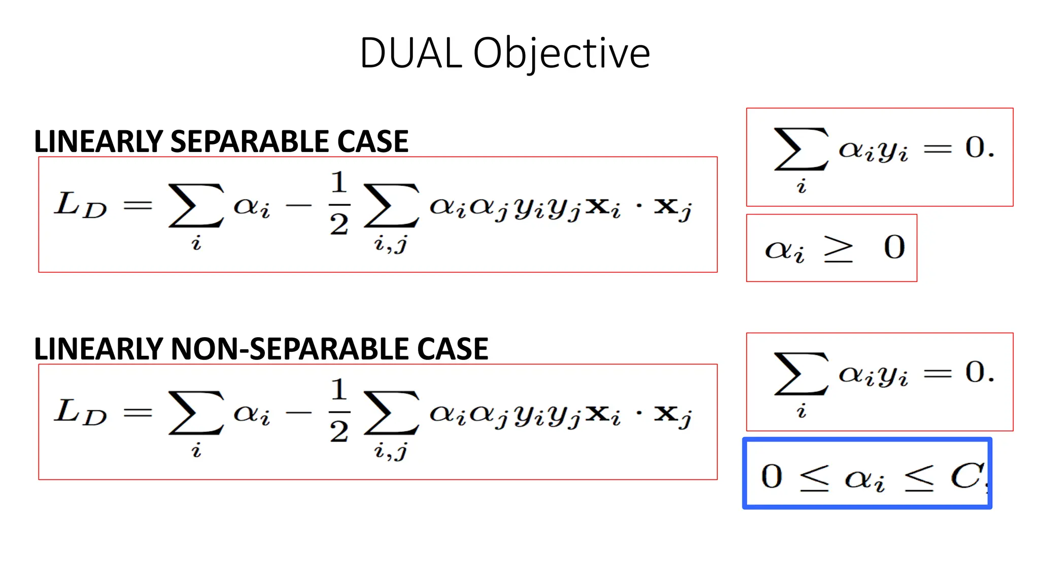
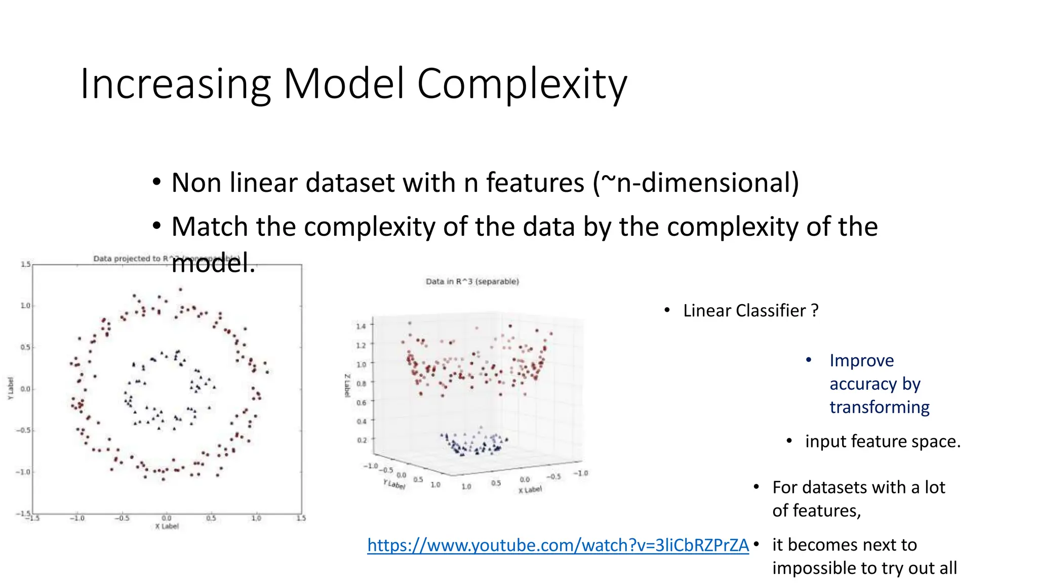
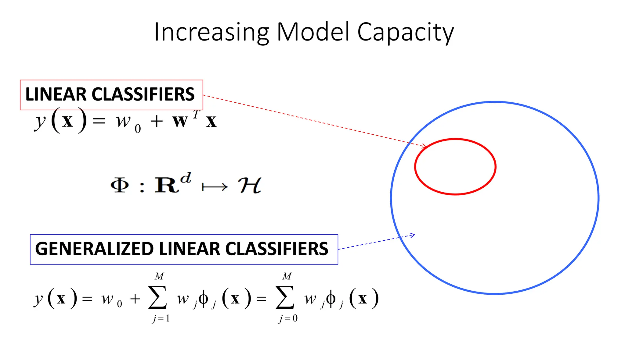
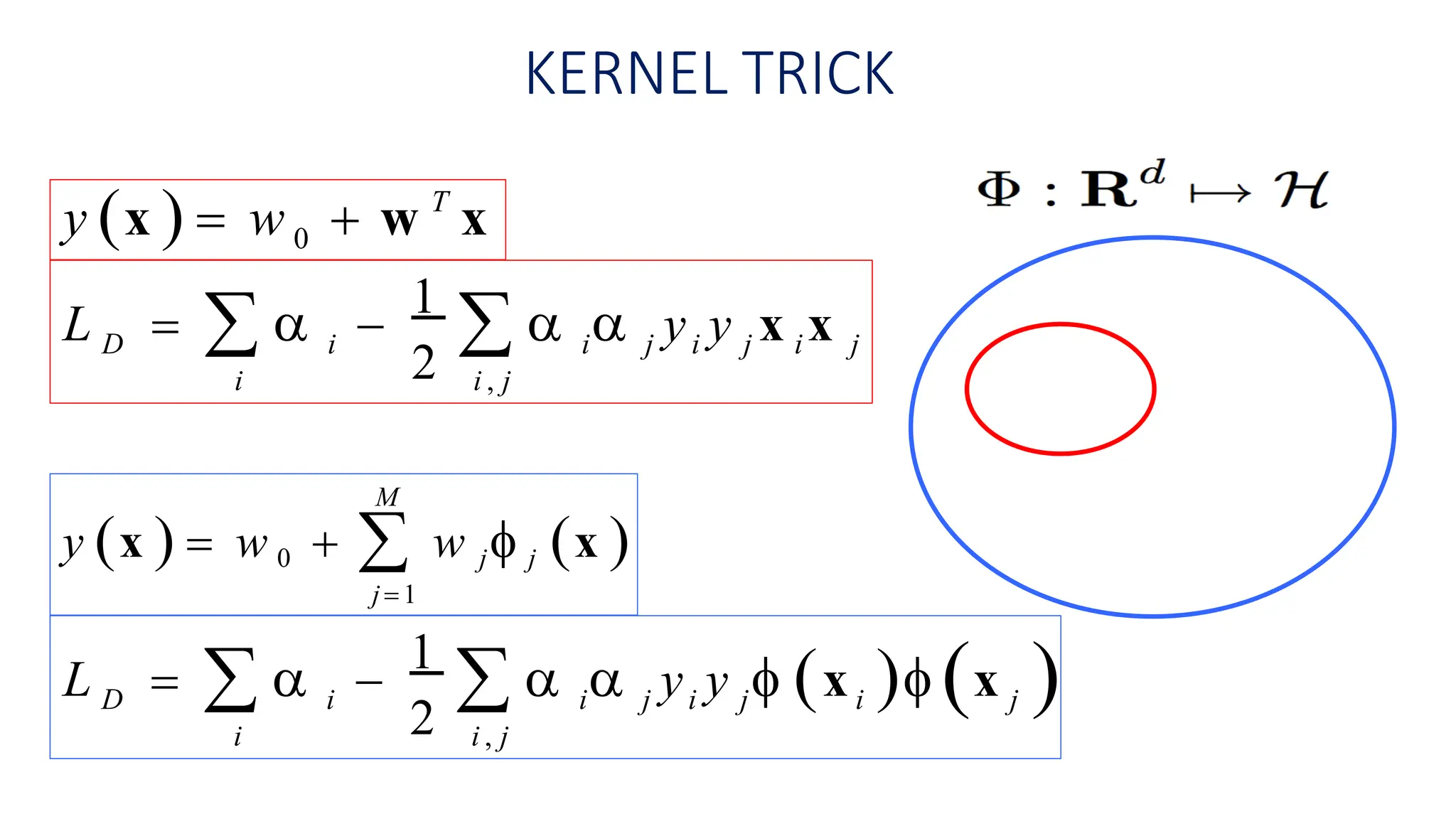
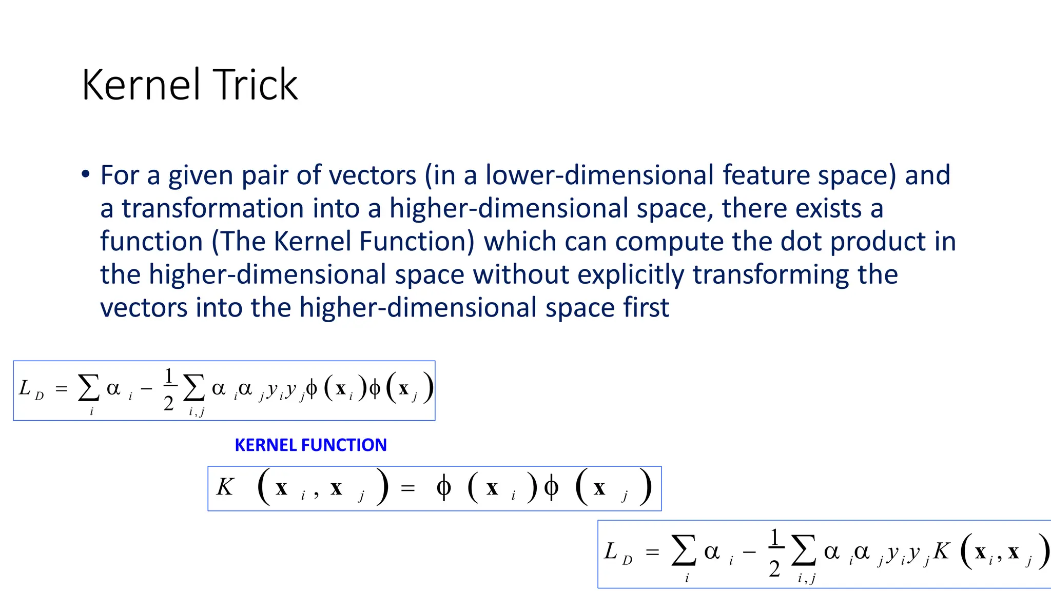
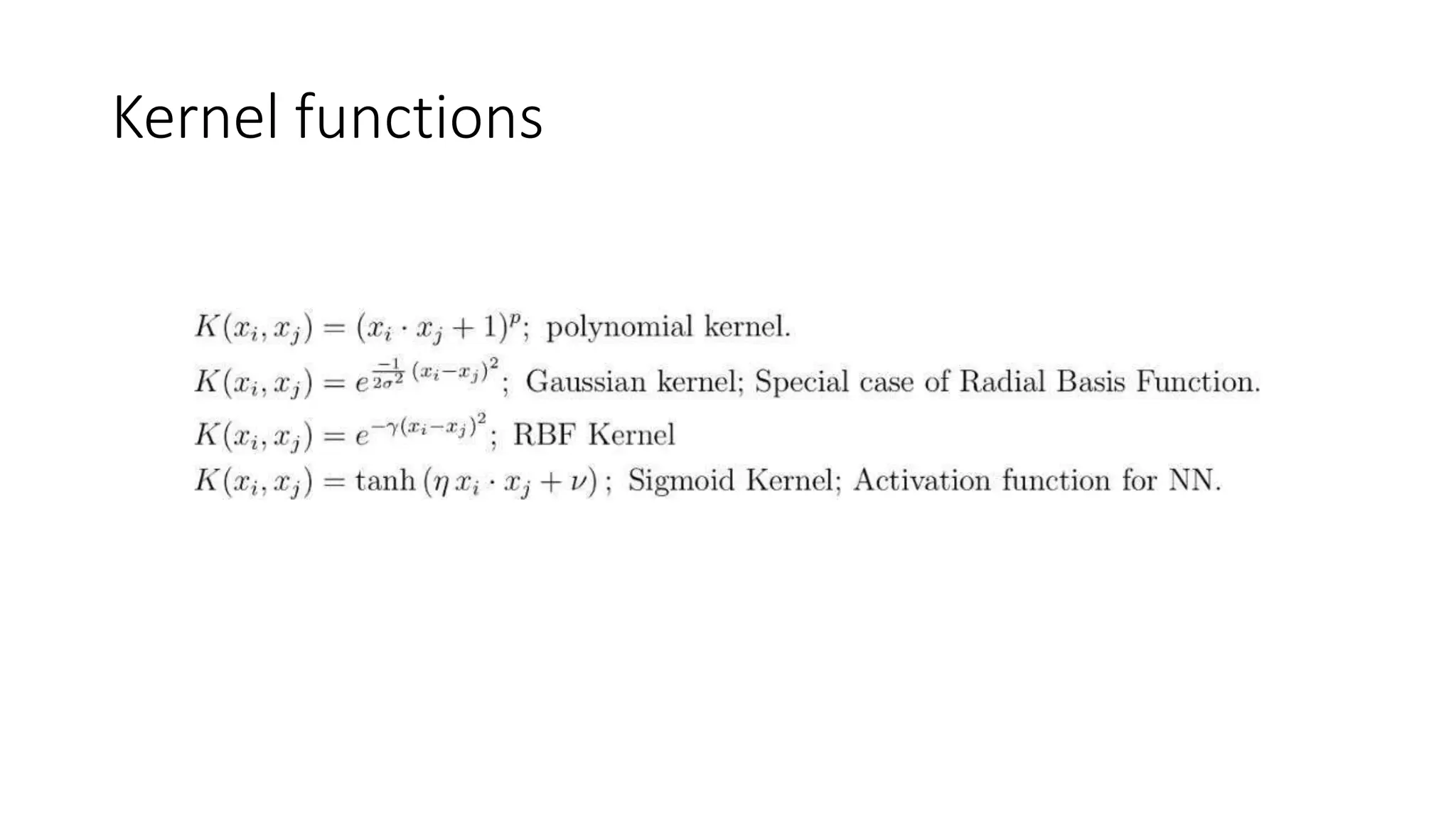
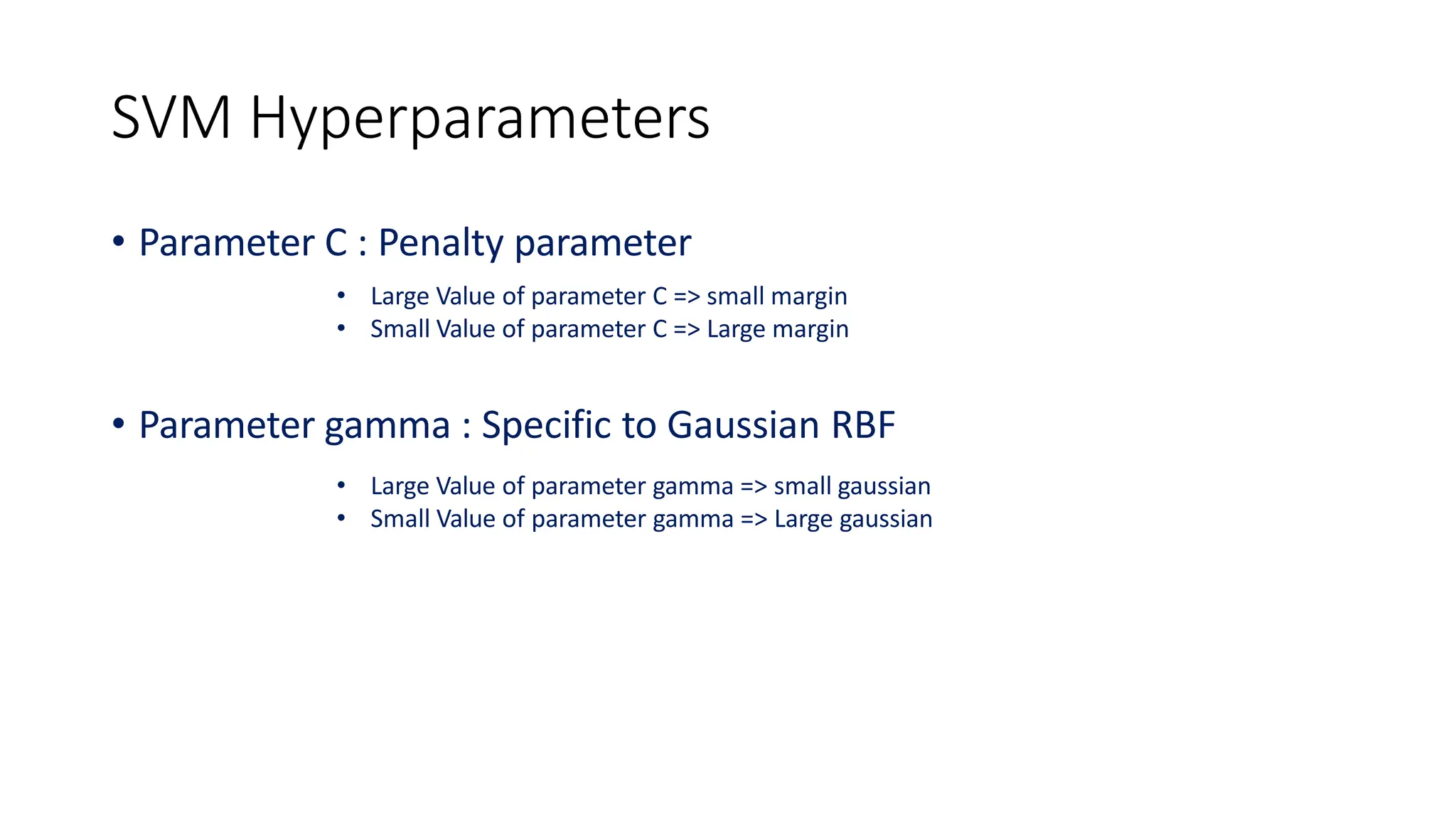
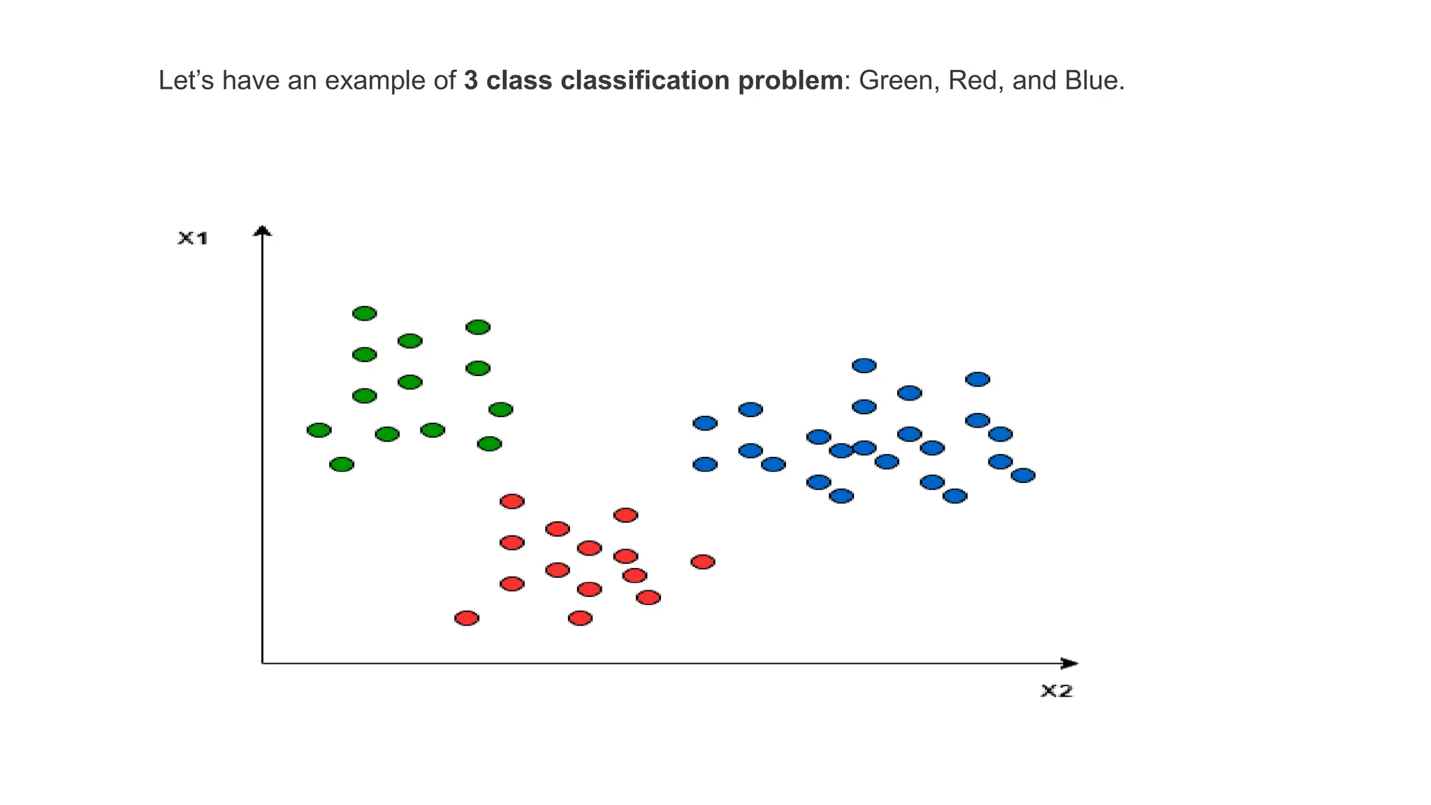
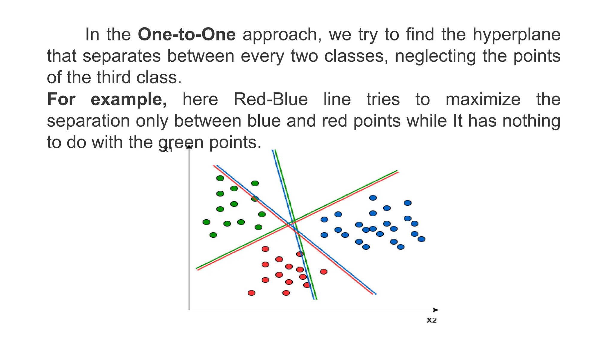
Support Vector Machines USING MACHINE LEARNING HOW IT WORKS

Support Vector Machines
Support Vector Machines: Overview, When Data is Linearly Separable, Support
Vector Classifier, When Data is NOT Linearly Separable, Kernel Functions,
Multiclass SVM.
Support Vector Machine (SVM) is one of the Machine Learning
(ML) Supervised algorithms. There are plenty of algorithms in
ML, but still, reception for SVM is always special because of its
strength while dealing with the data.

• This Support Vector Machine (SVM) presentation will help you
understand Support Vector Machine algorithm, a supervised
machine learning algorithm which can be used for both
classification and regression problems.
• This SVM presentation will help you learn where and when to
use SVM algorithm, how does the algorithm work, what are
hyperplanes and support vectors in SVM, how distance margin
helps in optimizing the hyperplane, kernel functions in SVM for
data transformation and advantages of SVM algorithm.
• At the end, we will also implement Support Vector Machine
algorithm in Python to differentiate crocodiles from alligators for
a given dataset.

• SVM is a supervised machine learning
algorithm that helps in
both classification and regression problem
statements.
• It tries to find an optimal boundary (known as
hyperplane) between different classes.
• In simple words, SVM does complex data
transformations depending on the selected kernel
function, and based on those transformations, it
aims to maximize the separation boundaries
between your data points.

Working of SVM:
• In the simplest form where there is a linear separation,
SVM tries to find a line that maximizes the separation
between a two-class data set of 2-dimensional space
points.
• The objective of SVM: The objective of SVM is to find
a hyperplane that maximizes the separation of the data
points to their actual classes in an n-dimensional space.
• The data points which are at the minimum distance to
the hyperplane i.e, closest points are called Support
Vectors.
• For Example, For the given diagram, the three points that are
layered on the scattered lines are the Support Vectors (2 blue

Why learn Machine Learning?
• Machine Learning is taking over the world- and with that, there
is a growing need among companies for professionals to know
the ins and outs of Machine Learning
• The Machine Learning market size is expected to grow from
USD 1.03 Billion in 2016 to USD 10.81 Billion by 2025, at a
Compound Annual Growth Rate (CAGR) of 54.1% during the
forecast period.

AI / ML
Machine Learning
Using Computer algorithms to
uncover insights, determine
relationships , and make prediction
about future trends.
Artificial Intelligence
Enabling computer systems to perform
tasks that ordinarily requires human
intelligence.
We use machine learning methods to create AI systems.

Machine Learning Paradigms
• Unsupervised Learning
• Find structure in data. (Clusters, Density, Patterns)
• Supervised Learning
• Find mapping between features to labels

Support Vector Machine
• Supervised machine learning Algorithm.
• Can be used for Classification/Regression.
• Works well with small datasets

Classification
• Classification using SVM
• 2 class problem , linearly separable data

The “Best” Separation Boundary
This is the widest road that
separates the two groups

This is the widest margin
that separates the two
groups
Margin

The distance between the
points and the line are as
far as possible.
Margin

The distance between the
support vectors and the
line are as far as possible.
Margin
Support
Vectors

This hyperplane is an
optimal hyperplane
because it is as far as
possible from the support
vectors.
Maximum
Margin
Support
Vectors
Hyperplane

Decision Rule
+
+
-
-
w
u
Projection
• w : normal vector of
any length
• u : unknown vector
and we want to find it
belongs to which
class?
Then unknown vector
will be classified as +

Constraints
+
+
-
-
Constraint for
positive samples
+
Likewise for
negative samples -
-1
1
0

+
+
-
-
Combining Constraints
Constraint for positive samples
Constraint for negative samples
0
0
To bring above inequalities together we
introduce another variable
For support vectors

Width
+
+
-
-
w
On the equation above x+ and x− are in the
gutter (on hyperplanes maximizing the
separation).
Positive Samples
Likewise Negative
Samples

SVM Objective
+
+
-
-
w
OBJECTIVE:
CONSTRAINT:
(Minimize)
Constrained Optimization problem.

Lagrange Multipliers
Lagrangian
OBJECTIVE: CONSTRAINT:

Solving the PRIMAL
 L P
 w
 L P
 0
 b
 0
The normal vector w are
the linear combination of
support vectors

SVM Objective (DUAL)
OBJECTIVE: Minimize
CONSTRAINT: SVM objective will depend only on
the dot product of pairs of support
vector.

Decision Rule
So whether a new sample will be
on the right of the road depends
on the dot product of the
support vectors and the
unknown sample.

Points to Consider
• SVM problem is constrained minimization problem
• To find the widest road between different samples we just need to
consider dot products of support vectors .

Non-Separable
+
-
-
w
-
+
+
Slack Variables

PRIMAL Objective
LINEARLY SEPARABLE CASE
LINEARLY NON-SEPARABLE CASE

DUAL Objective
LINEARLY SEPARABLE CASE
LINEARLY NON-SEPARABLE CASE

Increasing Model Complexity
• Non linear dataset with n features (~n-dimensional)
• Match the complexity of the data by the complexity of the
model.
• Linear Classifier ?
• Improve
accuracy by
transforming
• input feature space.
• For datasets with a lot
of features,
• it becomes next to
impossible to try out all
https://www.youtube.com/watch?v=3liCbRZPrZA

Increasing Model Capacity
y x   w 0  w T
x
M M
y x   w 0   w j j x    w j j x 
j  1 j  0
LINEAR CLASSIFIERS
GENERALIZED LINEAR CLASSIFIERS

KERNEL TRICK
  0
T
y x  w  w x
M
y x   w 0   w j j x 
j  1
D
2
i i j i j i j
i i , j
L    
1
   y y  x  x 
D
2
i i j i j i j
i i , j
L    
1
   y y x x

Kernel Trick
• For a given pair of vectors (in a lower-dimensional feature space) and
a transformation into a higher-dimensional space, there exists a
function (The Kernel Function) which can compute the dot product in
the higher-dimensional space without explicitly transforming the
vectors into the higher-dimensional space first
D i
2 i j i j i j
i i , j
L    
1
   y y  x  x 
KERNEL FUNCTION
K x i , x j     x i   x j 
D i
2 i j i j i j
i i , j
L    
1
   y y K x , x 

SVM Hyperparameters
• Parameter C : Penalty parameter
• Large Value of parameter C => small margin
• Small Value of parameter C => Large margin
• Parameter gamma : Specific to Gaussian RBF
• Large Value of parameter gamma => small gaussian
• Small Value of parameter gamma => Large gaussian

Multiclass Classification Using SVM
In its most basic type, SVM doesn’t support multiclass
classification. For multiclass classification, the same principle is
utilized after breaking down the multi-classification problem into
smaller subproblems, all of which are binary classification
problems.
The popular methods which are used to perform multi-
classification on the problem statements using SVM are as
follows:
One vs One (OVO) approach
One vs All (OVA) approach
Directed Acyclic Graph (DAG) approach

One vs One (OVO)
This technique breaks down our multiclass
classification problem into subproblems which are binary
classification problems. So, after this strategy, we get
binary classifiers per each pair of classes. For final
prediction for any input use the concept of majority
voting along with the distance from the margin as
its confidence criterion.
The major problem with this approach is that we
have to train too many SVMs.

Let’s have Multi-class/ Multi-labels problems with L
categories, then:
For the (s, t)- th classifier:
– Positive Samples: all the points in class s ({ xi : s
∈ yi })
– Negative samples: all the points in class t ({ xi : t ∈ yi })
– fs, t(x): the decision value of this classifier
( large value of f s, t(x) ⇒ label s has a higher probability
than the label t )
– f t, s (x) = – f s, t(x)
– Prediction: f(x)= argmax s ( Σ t fs, t(x) )

Let’s have an example of 3 class classification problem: Green, Red, and Blue.

In the One-to-One approach, we try to find the hyperplane
that separates between every two classes, neglecting the points
of the third class.
For example, here Red-Blue line tries to maximize the
separation only between blue and red points while It has nothing
to do with the green points.

One vs All (OVA)
In this technique, if we have N class problem, then
we learn N SVMs:
SVM number -1 learns “class_output = 1” vs
“class_output ≠ 1″
SVM number -2 learns “class_output = 2” vs
“class_output ≠ 2″
:
SVM number -N learns “class_output = N” vs
“class_output ≠ N”

Then to predict the output for new input, just predict with each of the
build SVMs and then find which one puts the prediction the farthest
into the positive region (behaves as a confidence criterion for a
particular SVM).
Now, a very important comes to mind that “Are there any
challenges in training these N SVMs?”
Yes, there are some challenges to train these N SVMs, which are:
1. Too much Computation: To implement the OVA strategy, we
require more training points which increases our computation.
2. Problems becomes Unbalanced: Let’s you are working on
an MNIST dataset, in which there are 10 classes from 0 to 9 and if we
have 1000 points per class, then for any one of the SVM having two
classes, one class will have 9000 points and other will have only
1000 data points, so our problem becomes unbalanced.

Now, how to address this unbalanced problem?
You have to take some representative (subsample) from
the class which is having more training samples i.e,
majority class. You can do this by using some below-listed
techniques:
– Use the 3-sigma rule of the normal distribution: Fit
data to a normal distribution and then subsampled
accordingly so that class distribution is maintained.
– Pick some data points randomly from the majority class.
– Use a popular subsampling technique named SMOTE.
Let’s have Multi-class/ multi-labels problems with L
categories, then:
For the t -th classifier:

– Positive Samples: all the points in class t ({ xi : t ∈ yi })
– Negative samples: all the points not in class t ({ xi : t ∉ yi })
– ft(x): the decision value for the t -th classifier.
( large value of ft ⇒ higher probability that x is in the class t)
– Prediction: f(x) = argmax t ft(x)
In the One vs All approach, we try to find a hyperplane to
separate the classes. This means the separation takes all points
into account and then divides them into two groups in which there is
a group for the one class points and the other group for all other
points.

For example, here, the Greenline tries to maximize the gap between green points and all other
points at once.
NOTE: A single SVM does binary
classification and can differentiate between
two classes. So according to the two above
approaches, to classify the data points from
L classes data set:
In the One vs All approach, the classifier
can use L SVMs.
In the One vs One approach, the classifier
can use L(L-1)/2 SVMs.

Directed Acyclic Graph (DAG)
This approach is more hierarchical in nature and it tries to
addresses the problems of the One vs One and One vs All approach.
This is a graphical approach in which we group the classes
based on some logical grouping.
Benefits: Benefits of this approach includes a fewer number of
SVM trains with respect to the OVA approach and it reduces the
diversity from the majority class which is a problem of the OVA
approach.
Problem: If we have given the dataset itself in the form of
different groups ( e.g, cifar 10 image classification dataset ) then
we can directly apply this approach but if we don’t give the groups,
then the problem with this approach is of finding the logical grouping
in the dataset i.e, we have to manually pick the logical grouping.

The advantages of support vector machines are:
• Effective in high dimensional spaces.
• Still effective in cases where number of dimensions is greater
than the number of samples.
• Uses a subset of training points in the decision function (called
support vectors), so it is also memory efficient.
• Versatile: different Kernel functions can be specified for the
decision function. Common kernels are provided, but it is also
possible to specify custom kernels.
The disadvantages of support vector machines include:
• If the number of features is much greater than the number of
samples, avoid over-fitting in choosing Kernel functions and
regularization term is crucial.
• SVMs do not directly provide probability estimates, these are
calculated using an expensive five-fold cross-validation

Source
• https://www.quora.com/What-are-C-and-gamma-with-regards-to-a-support-vector-
machine
• https://www.quora.com/How-can-I-choose-the-parameter-C-for-SVM
• https://www.youtube.com/watch?v=_PwhiWxHK8o
• https://www.youtube.com/watch?v=N1vOgolbjSc
• https://medium.com/@pushkarmandot/what-is-the-significance-of-c-value-in-support-
vector-machine-28224e852c5a
• https://towardsdatascience.com/understanding-support-vector-machine-part-1-
lagrange-multipliers-5c24a52ffc5e
• https://towardsdatascience.com/understanding-support-vector-machine-part-2-kernel-
trick-mercers-theorem-e1e6848c6c4d
• http://web.mit.edu/6.034/wwwbob/svm-notes-long-08.pdf
• https://www.quora.com/What-is-the-kernel-trick

Support Vector Machines USING MACHINE LEARNING HOW IT WORKS

Recommended

Recommended

More Related Content

Similar to Support Vector Machines USING MACHINE LEARNING HOW IT WORKS

Similar to Support Vector Machines USING MACHINE LEARNING HOW IT WORKS (20)

More from rajalakshmi5921

More from rajalakshmi5921 (20)

Recently uploaded

Recently uploaded (20)

Support Vector Machines USING MACHINE LEARNING HOW IT WORKS