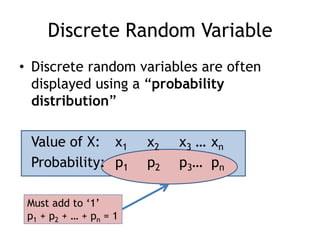
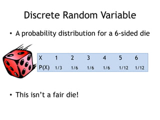
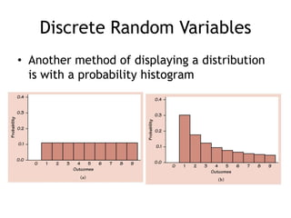
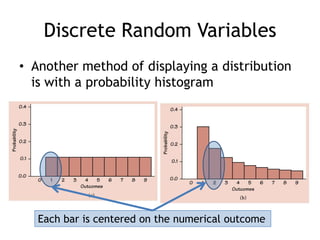
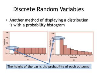
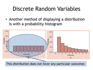
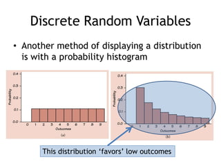
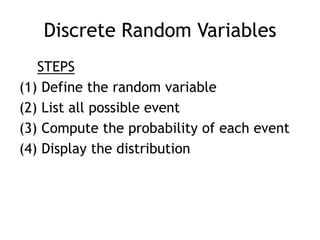
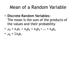
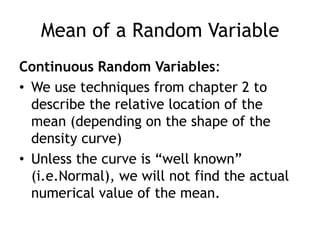
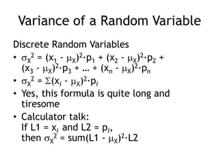
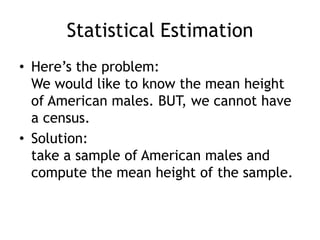
Chapter 7Random Variables
7.1 Discrete and Continuous Random Variables
Random Variables	A random variable is a variable whose value is a numerical outcome of a random phenomenonex1 The sum of the pips on two diceex2 The net gain or loss after a game of blackjackex3 The amount of soda in a cup from a vending machine
Discrete Random VariableFor a discrete random variable X, the number of outcomes is countable (finite)Ex3 (the soda from a vending machine) is not discrete.  Why?
Discrete Random VariableDiscrete random variables are often displayed using a “probability distribution”	Value of X:	x1	x2	x3 …	xnProbability:	p1	p2	p3…	pn
Discrete Random VariableDiscrete random variables are often displayed using a “probability distribution”	Value of X:	x1	x2	x3 …	xnProbability:	p1	p2	p3…	pnP(X=x1)=p1“Probability that X = x1 is p1”
Discrete Random VariableDiscrete random variables are often displayed using a “probability distribution”	Value of X:	x1	x2	x3 …	xnProbability:	p1	p2	p3…	pnMust add to ‘1’p1 + p2 + … + pn = 1
Discrete Random VariableA probability distribution for a 6-sided dieThis isn’t a fair die!X	1	2	3	4	5	6P(X)	1/3	1/6	1/6	1/6	1/12	1/12
Discrete Random VariablesAnother method of displaying a distribution is with a probability histogram
Discrete Random VariablesAnother method of displaying a distribution is with a probability histogramEach bar is centered on the numerical outcome
Discrete Random VariablesAnother method of displaying a distribution is with a probability histogramThe height of the bar is the probability of each outcome
Discrete Random VariablesAnother method of displaying a distribution is with a probability histogramThis distribution does not favor any particular outcomes
Discrete Random VariablesAnother method of displaying a distribution is with a probability histogramThis distribution ‘favors’ low outcomes
Discrete Random VariablesSTEPS Define the random variable List all possible eventCompute the probability of each event Display the distribution
Discrete Random VariablesLet look at the probability distribution for the number of ‘heads’ produced by flipping two fair coins
Discrete Random Variables Define the random variable	“Let X = the number of heads produced by flipping two fair coins”
Discrete Random Variables(2) List all possible outcomesRemember that each coin is independentTip: be systematic when listing outcomesLet’s look at the outcomes that have ‘0 heads’	TT		there’s only one of these
Discrete Random VariablesHow many outcomes have ‘1 heads’HTTHtwo outcomes!
Discrete Random VariablesHow many outcomes have ‘2 heads’HHonly one outcomeThere were 4 equally likely outcomes
Discrete Random Variables(3) Compute the probability of each event	“# outcomes for event/# of outcomes	P(X = 0) = ¼	P(X = 1) = 2/4 = ½ 	P(X = 2) = ¼
Discrete Random Variables(4) Display the distributionProbability Distribution
Discrete Random Variables(4) Display the distributionProbability Histogram.6.4.20	1	2	3
Continuous Random VariablesUnlike the discrete random variable, a continuous random variable has an uncountable number of outcomesA continuous random variable X takes on all values in an interval of numbers
Continuous Random VariablesThe probability distribution for a continuous rand var is described/ displayed with a density curve.The probability of an event is the area under the density curve and above the values of X that make up the eventThe area under a density curve is ‘1’A density curve lies above the x-axis at all points.
Continuous Random VariablesThese distributions are called “uniform”
Continuous Random Variables
Continuous Random VariablesCuriously, since there is no area above any single value of x, P(X = x) = 0 for all values of x
Continuous Random VariablesThe Normal distribution is also a density curve!P( - < z < ) = 1If a random variable can be transformed into the Normal distribution, we can use methods we learned earlier to compute probability!
Continuous Random VariablesEXAMPLE		A soda machine dispenses soda into a 12 oz paper cup.  The amount of soda dispensed  if Normal with  = 11.8 oz and  = 0.14 oz.  What proportion of cups dispensed are between 11.7 and 12 ozs?
Continuous Random VariablesRemember these:State problem in terms of ‘x,’ the observed variable.  Draw and shade the distribution of ‘x.’Standardize (find the z-score).  Use proper notation!Draw and shade the Normal distribution.Find the area using Table A or your calculator.Remember that the area under curve is ‘1.’Write up a conclusion in context of the problem.
Continuous Random Variables(1) This time, we define our random variable X.“Let X = the amount of soda dispensed into a cup.”		         11.66  	11.8     11.94		 	11.7		  12
Continuous Random Variables(2)Standardize (find the z-score).  Draw and shade the Normal distribution.		 	    -0.71		  1.43
Continuous Random Variables(3) Find the area using Table A or your calculator.Remember that the area under curve is ‘1.’	P(-0.71<z<1.43) = 0.6848(4) Write up a conclusion in context of the problem.“The proportion of cups whose volume of soda is between 11.7 and 12 ozs is 0.6848”
7.2 Means and variances of random variables
Mean of a Random VariableSymbol is ‘mu’ (again)This mean is often called the “expected value” ExThe expected value does not have to be a possible value of X because it describes behavior over the long run
Mean of a Random VariableDiscrete Random Variables:The mean is the sum of the products of the values and their probabilityX = x1p1 + x2p2 + x3p3 + … + xnpnX = xipi
Mean of a Random VariableContinuous Random Variables:We use techniques from chapter 2 to describe the relative location of the mean (depending on the shape of the density curve)Unless the curve is “well known” (i.e.Normal), we will not find the actual numerical value of the mean.
Variance of a Random VariableDiscrete Random VariablesX2 = (x1 - X)2·p1 + (x2 - X)2·p2 + (x3 - X)2·p3 + … + (xn - X)2·pnX2 = (xi - X)2·piYes, this formula is quite long and tiresomeCalculator talk:If L1 = xi  and L2 = pi, then X2 = sum(L1 - X)2·L2
Statistical EstimationHere’s the problem:We would like to know the mean height of American males. BUT, we cannot have a census.Solution:take a sample of American males and compute the mean height of the sample.
Statistical EstimationSuppose we took many samples.The histogram for the means of the samples will have it’s own distributionremember, this is the distribution of the means of the samples, and not the distribution of the heights of American malesThis distribution of the samples is called a “sampling distribution”
The Law of Large NumbersFor any distribution, as the number of observations increases in the sample, the sample mean (Xbar) will approach the population mean .This is true for all distributions, not just Normal distributions.
The Law of Large Numbers	Remember the following for random behavior:Behavior in the short run is unpredictableBehavior in the long run is regular and predictableThis is the Law of Large Numbers	This begs the question, how many observations is “the long run?”
Transformations for MeansIf a random variable undergoes a linear transformation to form a new random variable, Then the mean of the new random variable undergoes the same transformation.If:		 X2 = a + bX1Then:	X2 = a + b X1
Combining Two MeansIf two random variables are added/subtracted to for a new random variable, Then the mean of the new random variable is the two means added/subtractedIF: 		X = X1 ± X2Then	X = X1± X2
Transformations for VarianceIf a random variable undergoes a linear transformation, Then the variance of the new random variable is the product of the square of the multiplier and the old varianceIf:		 X2 = a + bX1Then:	 (X2)2 = b2· (X1)2Std Dev is the square root of variance
Combining Two VariancesIf two random variables are added/subtracted to for a new random variable, Then the variance of the new random variable is the sum of the squares of the old variancesIF: 		X = X1 ± X2Then	 (X)2 = (X1)2+ (X2)2ALWAYS ADD VARIANCESStd Dev is the square root of variance
Normal Random VariablesAny linear combination or transformation of Normal random variables is also Normal.IMPORTANT: you must state that a distribution is Normal before you can use techniques for Normal density curves.Especially true after a linear combination or transformation.
WILSON!!!!It’s doubtful that this is Normal behavior

Stats chapter 7

  • 1.
  • 2.
    7.1 Discrete andContinuous Random Variables
  • 3.
    Random Variables A randomvariable is a variable whose value is a numerical outcome of a random phenomenonex1 The sum of the pips on two diceex2 The net gain or loss after a game of blackjackex3 The amount of soda in a cup from a vending machine
  • 4.
    Discrete Random VariableFora discrete random variable X, the number of outcomes is countable (finite)Ex3 (the soda from a vending machine) is not discrete. Why?
  • 5.
    Discrete Random VariableDiscreterandom variables are often displayed using a “probability distribution” Value of X: x1 x2 x3 … xnProbability: p1 p2 p3… pn
  • 6.
    Discrete Random VariableDiscreterandom variables are often displayed using a “probability distribution” Value of X: x1 x2 x3 … xnProbability: p1 p2 p3… pnP(X=x1)=p1“Probability that X = x1 is p1”
  • 7.
    Discrete Random VariableDiscreterandom variables are often displayed using a “probability distribution” Value of X: x1 x2 x3 … xnProbability: p1 p2 p3… pnMust add to ‘1’p1 + p2 + … + pn = 1
  • 8.
    Discrete Random VariableAprobability distribution for a 6-sided dieThis isn’t a fair die!X 1 2 3 4 5 6P(X) 1/3 1/6 1/6 1/6 1/12 1/12
  • 9.
    Discrete Random VariablesAnothermethod of displaying a distribution is with a probability histogram
  • 10.
    Discrete Random VariablesAnothermethod of displaying a distribution is with a probability histogramEach bar is centered on the numerical outcome
  • 11.
    Discrete Random VariablesAnothermethod of displaying a distribution is with a probability histogramThe height of the bar is the probability of each outcome
  • 12.
    Discrete Random VariablesAnothermethod of displaying a distribution is with a probability histogramThis distribution does not favor any particular outcomes
  • 13.
    Discrete Random VariablesAnothermethod of displaying a distribution is with a probability histogramThis distribution ‘favors’ low outcomes
  • 14.
    Discrete Random VariablesSTEPSDefine the random variable List all possible eventCompute the probability of each event Display the distribution
  • 15.
    Discrete Random VariablesLetlook at the probability distribution for the number of ‘heads’ produced by flipping two fair coins
  • 16.
    Discrete Random VariablesDefine the random variable “Let X = the number of heads produced by flipping two fair coins”
  • 17.
    Discrete Random Variables(2)List all possible outcomesRemember that each coin is independentTip: be systematic when listing outcomesLet’s look at the outcomes that have ‘0 heads’ TT there’s only one of these
  • 18.
    Discrete Random VariablesHowmany outcomes have ‘1 heads’HTTHtwo outcomes!
  • 19.
    Discrete Random VariablesHowmany outcomes have ‘2 heads’HHonly one outcomeThere were 4 equally likely outcomes
  • 20.
    Discrete Random Variables(3)Compute the probability of each event “# outcomes for event/# of outcomes P(X = 0) = ¼ P(X = 1) = 2/4 = ½ P(X = 2) = ¼
  • 21.
    Discrete Random Variables(4)Display the distributionProbability Distribution
  • 22.
    Discrete Random Variables(4)Display the distributionProbability Histogram.6.4.20 1 2 3
  • 23.
    Continuous Random VariablesUnlikethe discrete random variable, a continuous random variable has an uncountable number of outcomesA continuous random variable X takes on all values in an interval of numbers
  • 24.
    Continuous Random VariablesTheprobability distribution for a continuous rand var is described/ displayed with a density curve.The probability of an event is the area under the density curve and above the values of X that make up the eventThe area under a density curve is ‘1’A density curve lies above the x-axis at all points.
  • 25.
    Continuous Random VariablesThesedistributions are called “uniform”
  • 26.
  • 27.
    Continuous Random VariablesCuriously,since there is no area above any single value of x, P(X = x) = 0 for all values of x
  • 28.
    Continuous Random VariablesTheNormal distribution is also a density curve!P( - < z < ) = 1If a random variable can be transformed into the Normal distribution, we can use methods we learned earlier to compute probability!
  • 29.
    Continuous Random VariablesEXAMPLE Asoda machine dispenses soda into a 12 oz paper cup. The amount of soda dispensed if Normal with  = 11.8 oz and  = 0.14 oz. What proportion of cups dispensed are between 11.7 and 12 ozs?
  • 30.
    Continuous Random VariablesRememberthese:State problem in terms of ‘x,’ the observed variable. Draw and shade the distribution of ‘x.’Standardize (find the z-score). Use proper notation!Draw and shade the Normal distribution.Find the area using Table A or your calculator.Remember that the area under curve is ‘1.’Write up a conclusion in context of the problem.
  • 31.
    Continuous Random Variables(1)This time, we define our random variable X.“Let X = the amount of soda dispensed into a cup.” 11.66 11.8 11.94 11.7 12
  • 32.
    Continuous Random Variables(2)Standardize(find the z-score). Draw and shade the Normal distribution. -0.71 1.43
  • 33.
    Continuous Random Variables(3)Find the area using Table A or your calculator.Remember that the area under curve is ‘1.’ P(-0.71<z<1.43) = 0.6848(4) Write up a conclusion in context of the problem.“The proportion of cups whose volume of soda is between 11.7 and 12 ozs is 0.6848”
  • 34.
    7.2 Means andvariances of random variables
  • 35.
    Mean of aRandom VariableSymbol is ‘mu’ (again)This mean is often called the “expected value” ExThe expected value does not have to be a possible value of X because it describes behavior over the long run
  • 36.
    Mean of aRandom VariableDiscrete Random Variables:The mean is the sum of the products of the values and their probabilityX = x1p1 + x2p2 + x3p3 + … + xnpnX = xipi
  • 37.
    Mean of aRandom VariableContinuous Random Variables:We use techniques from chapter 2 to describe the relative location of the mean (depending on the shape of the density curve)Unless the curve is “well known” (i.e.Normal), we will not find the actual numerical value of the mean.
  • 38.
    Variance of aRandom VariableDiscrete Random VariablesX2 = (x1 - X)2·p1 + (x2 - X)2·p2 + (x3 - X)2·p3 + … + (xn - X)2·pnX2 = (xi - X)2·piYes, this formula is quite long and tiresomeCalculator talk:If L1 = xi and L2 = pi, then X2 = sum(L1 - X)2·L2
  • 39.
    Statistical EstimationHere’s theproblem:We would like to know the mean height of American males. BUT, we cannot have a census.Solution:take a sample of American males and compute the mean height of the sample.
  • 40.
    Statistical EstimationSuppose wetook many samples.The histogram for the means of the samples will have it’s own distributionremember, this is the distribution of the means of the samples, and not the distribution of the heights of American malesThis distribution of the samples is called a “sampling distribution”
  • 41.
    The Law ofLarge NumbersFor any distribution, as the number of observations increases in the sample, the sample mean (Xbar) will approach the population mean .This is true for all distributions, not just Normal distributions.
  • 42.
    The Law ofLarge Numbers Remember the following for random behavior:Behavior in the short run is unpredictableBehavior in the long run is regular and predictableThis is the Law of Large Numbers This begs the question, how many observations is “the long run?”
  • 43.
    Transformations for MeansIfa random variable undergoes a linear transformation to form a new random variable, Then the mean of the new random variable undergoes the same transformation.If: X2 = a + bX1Then: X2 = a + b X1
  • 44.
    Combining Two MeansIftwo random variables are added/subtracted to for a new random variable, Then the mean of the new random variable is the two means added/subtractedIF: X = X1 ± X2Then X = X1± X2
  • 45.
    Transformations for VarianceIfa random variable undergoes a linear transformation, Then the variance of the new random variable is the product of the square of the multiplier and the old varianceIf: X2 = a + bX1Then: (X2)2 = b2· (X1)2Std Dev is the square root of variance
  • 46.
    Combining Two VariancesIftwo random variables are added/subtracted to for a new random variable, Then the variance of the new random variable is the sum of the squares of the old variancesIF: X = X1 ± X2Then (X)2 = (X1)2+ (X2)2ALWAYS ADD VARIANCESStd Dev is the square root of variance
  • 47.
    Normal Random VariablesAnylinear combination or transformation of Normal random variables is also Normal.IMPORTANT: you must state that a distribution is Normal before you can use techniques for Normal density curves.Especially true after a linear combination or transformation.
  • 48.
    WILSON!!!!It’s doubtful thatthis is Normal behavior