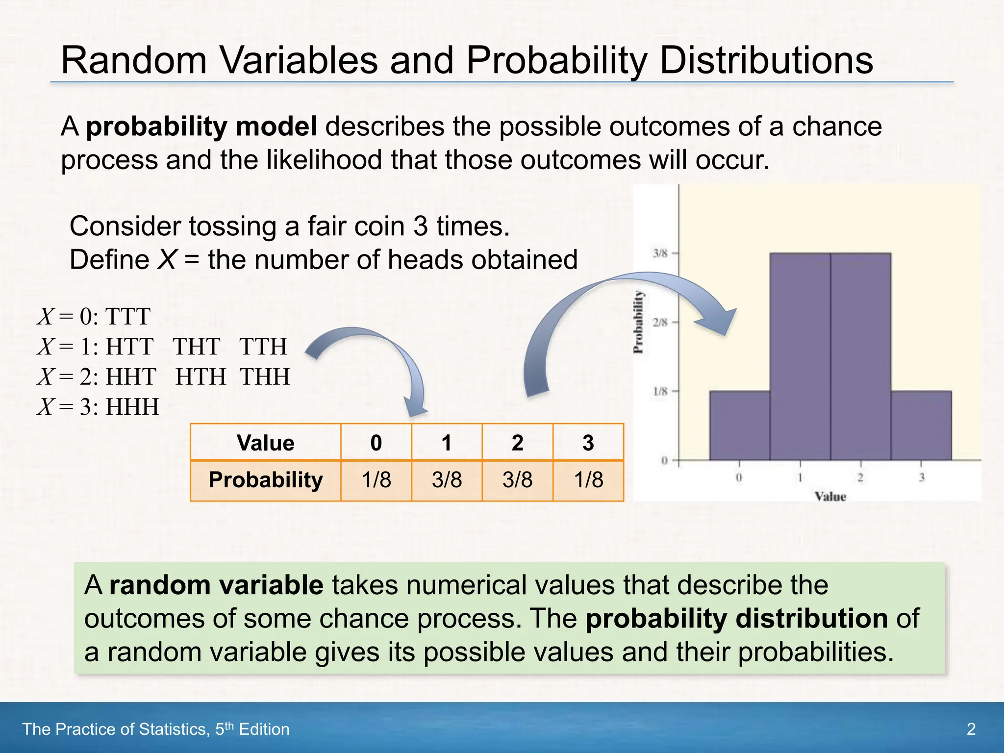
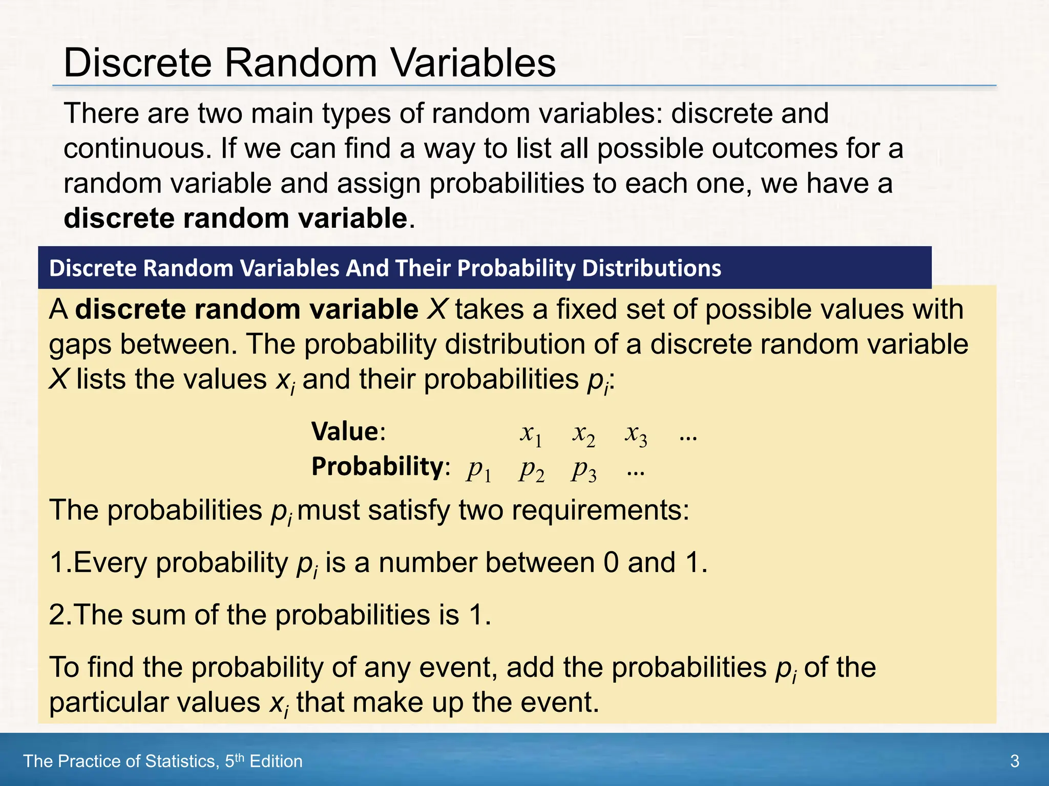
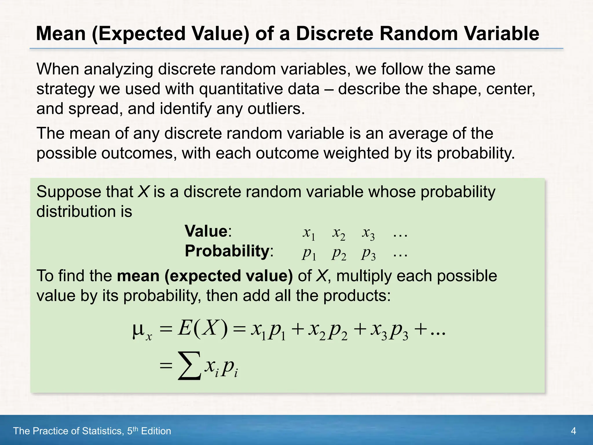
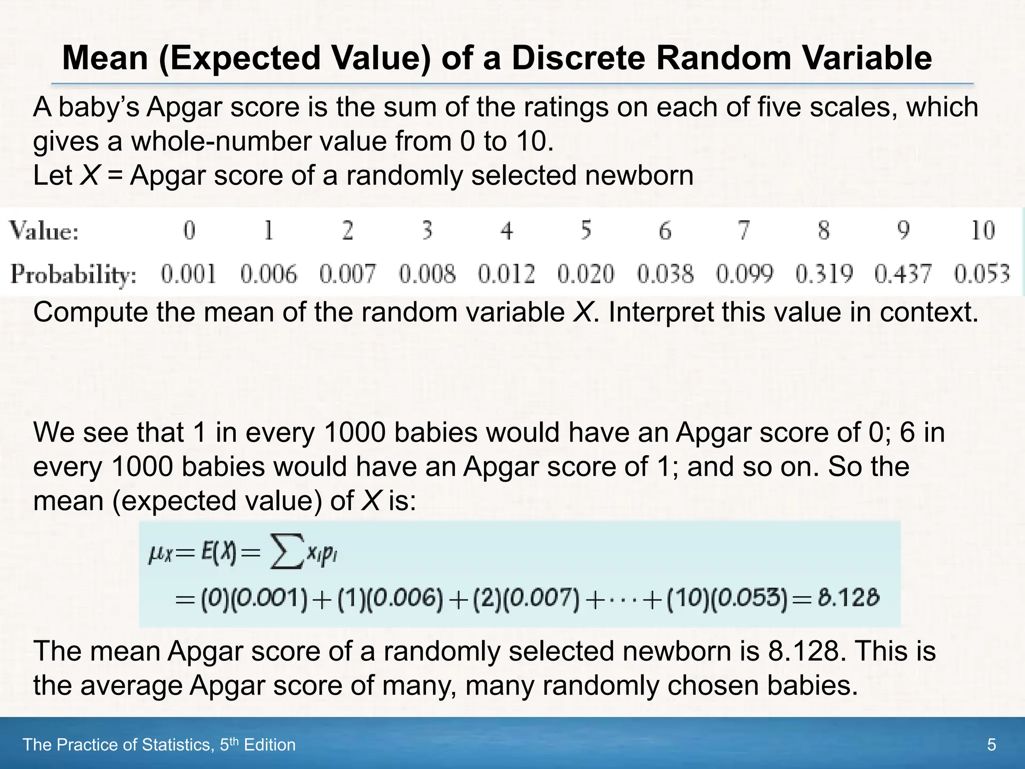
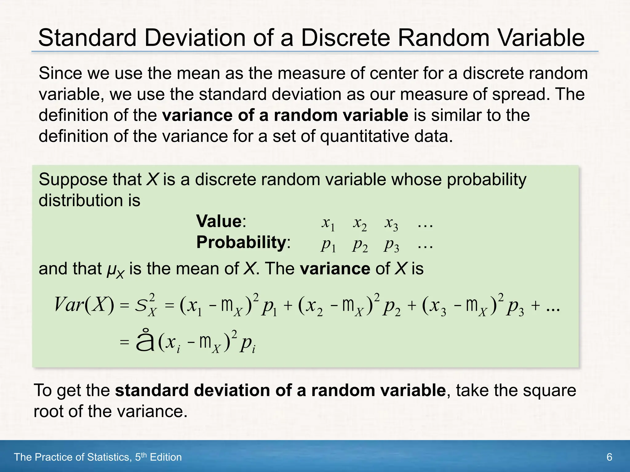
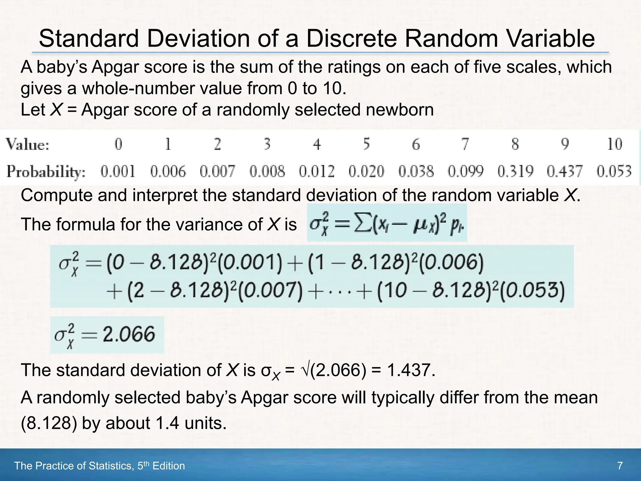
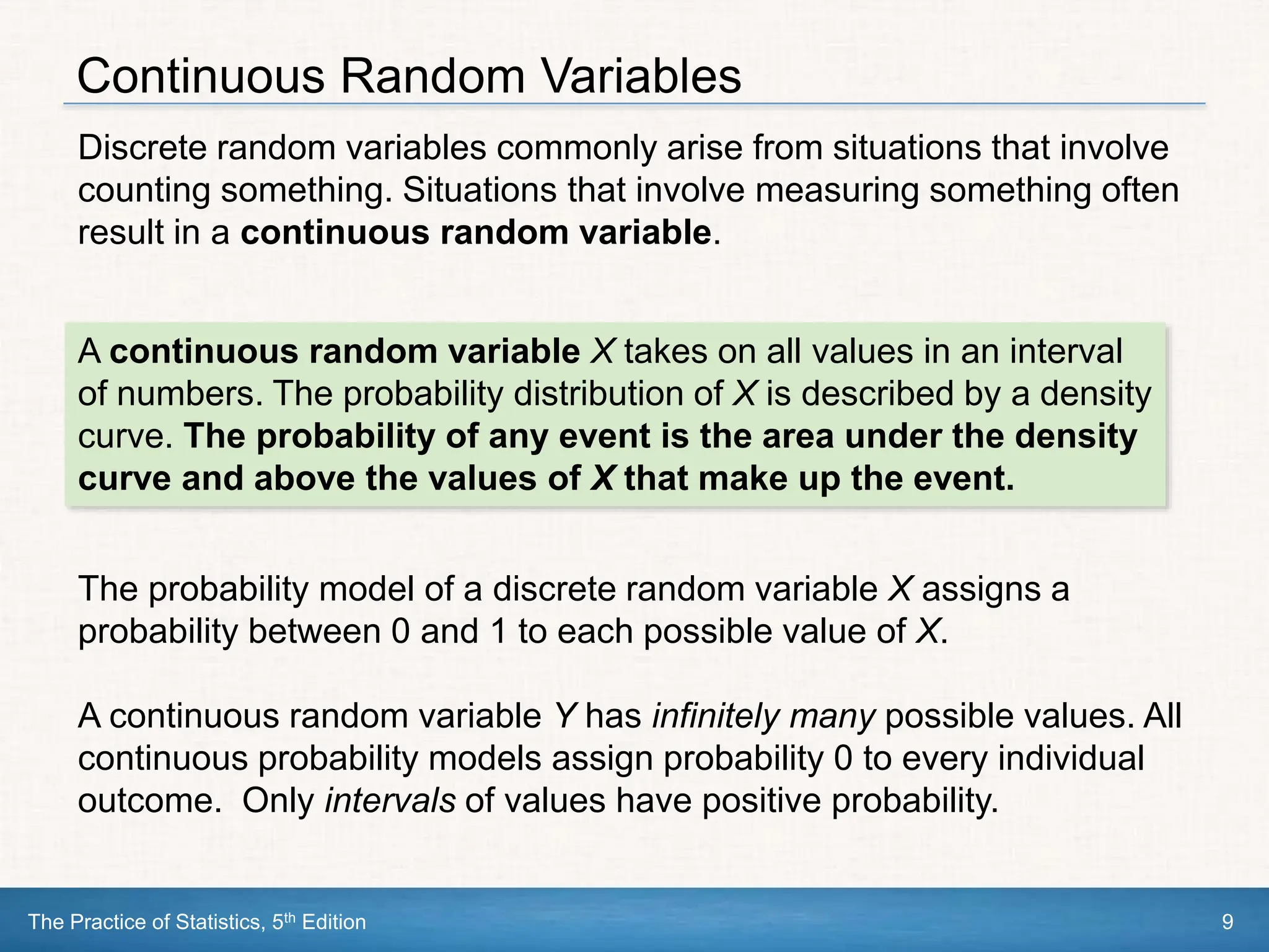
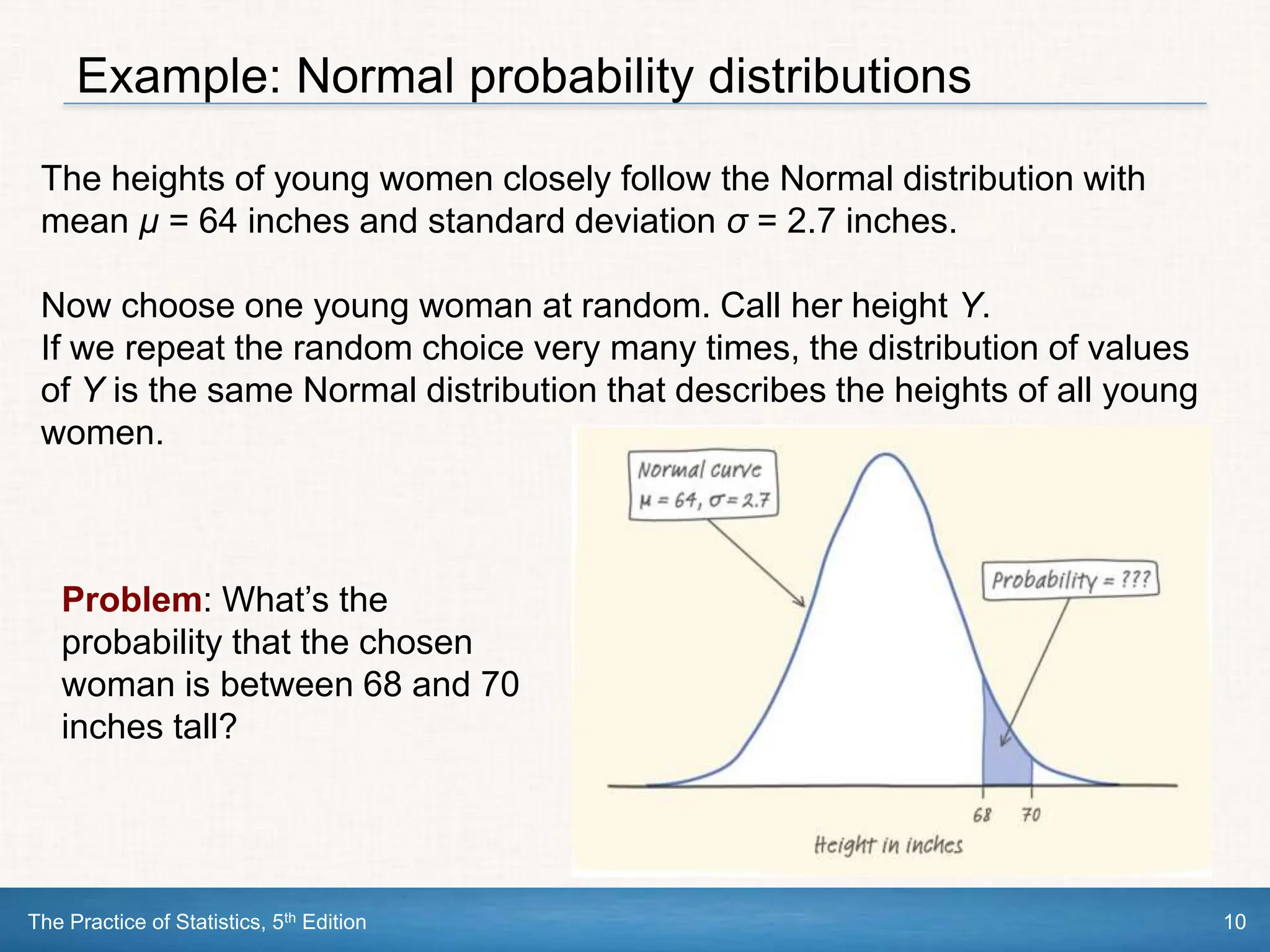
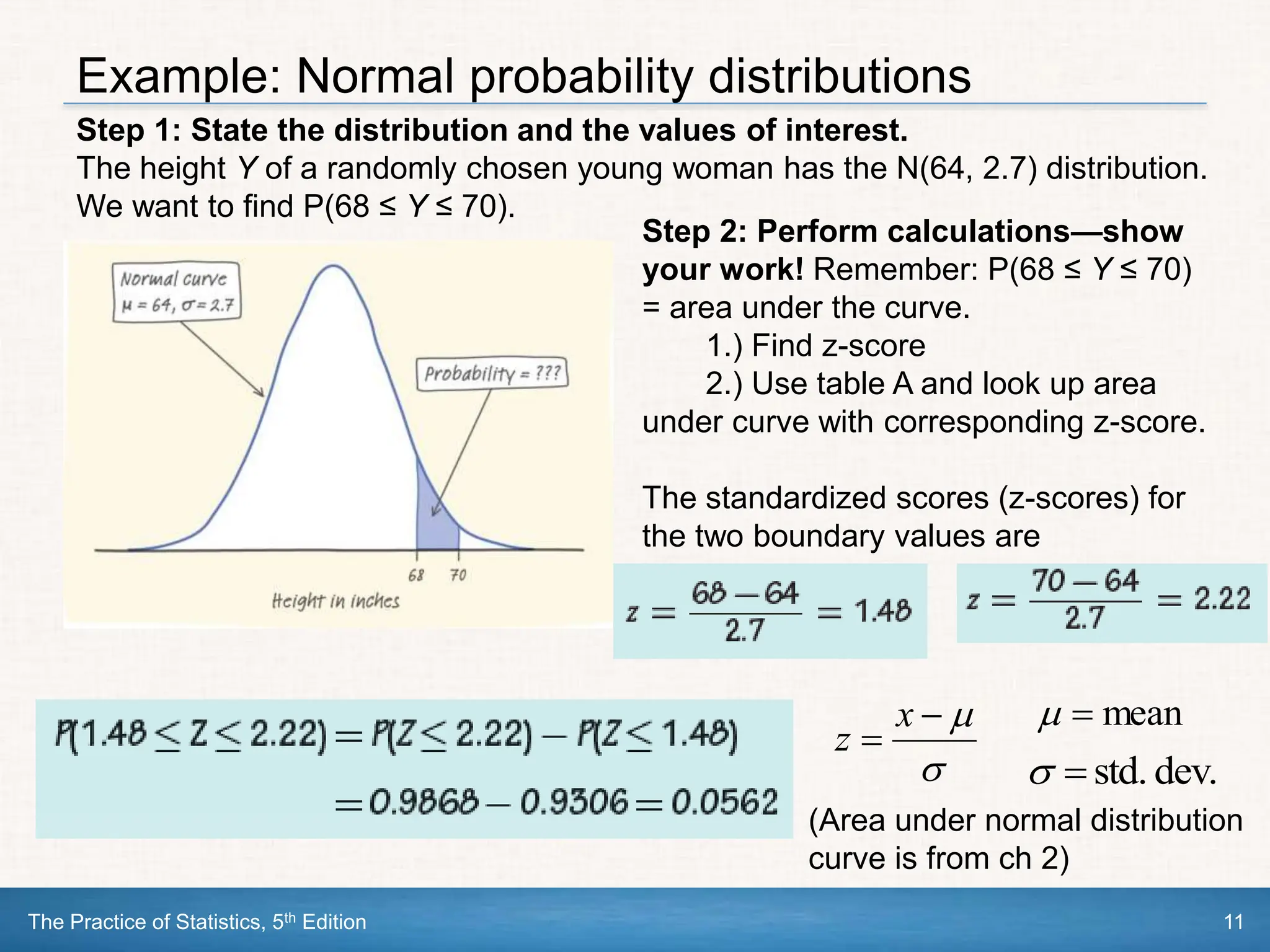
SlideShare a Scribd company logo
1 of 12
The Practice of Statistics, 5th Edition
Starnes, Tabor, Yates, Moore
Bedford Freeman Worth Publishers
CHAPTER 6
Random Variables
6.1: Discrete and Continuous
Random Variables
HW due Friday: p.359 (2, 3, 6, 8, 9, 11, 14,
15, 19, 21, 23, 26, 30)
Tutorial next week Tuesday for QM review
The Practice of Statistics, 5th Edition 2
Random Variables and Probability Distributions
A probability model describes the possible outcomes of a chance
process and the likelihood that those outcomes will occur.
A random variable takes numerical values that describe the
outcomes of some chance process. The probability distribution of
a random variable gives its possible values and their probabilities.
X = 0: TTT
X = 1: HTT THT TTH
X = 2: HHT HTH THH
X = 3: HHH
Value 0 1 2 3
Probability 1/8 3/8 3/8 1/8
Consider tossing a fair coin 3 times.
Define X = the number of heads obtained
The Practice of Statistics, 5th Edition 3
Discrete Random Variables
A discrete random variable X takes a fixed set of possible values with
gaps between. The probability distribution of a discrete random variable
X lists the values xi and their probabilities pi:
Value: x1 x2 x3 …
Probability: p1 p2 p3 …
The probabilities pi must satisfy two requirements:
1.Every probability pi is a number between 0 and 1.
2.The sum of the probabilities is 1.
To find the probability of any event, add the probabilities pi of the
particular values xi that make up the event.
Discrete Random Variables And Their Probability Distributions
There are two main types of random variables: discrete and
continuous. If we can find a way to list all possible outcomes for a
random variable and assign probabilities to each one, we have a
discrete random variable.
The Practice of Statistics, 5th Edition 4
Mean (Expected Value) of a Discrete Random Variable
When analyzing discrete random variables, we follow the same
strategy we used with quantitative data – describe the shape, center,
and spread, and identify any outliers.
The mean of any discrete random variable is an average of the
possible outcomes, with each outcome weighted by its probability.
Suppose that X is a discrete random variable whose probability
distribution is
Value: x1 x2 x3 …
Probability: p1 p2 p3 …
To find the mean (expected value) of X, multiply each possible
value by its probability, then add all the products:








i
i
x
p
x
p
x
p
x
p
x
X
E ...
)
( 3
3
2
2
1
1
The Practice of Statistics, 5th Edition 5
Mean (Expected Value) of a Discrete Random Variable
A baby’s Apgar score is the sum of the ratings on each of five scales, which
gives a whole-number value from 0 to 10.
Let X = Apgar score of a randomly selected newborn
Compute the mean of the random variable X. Interpret this value in context.
We see that 1 in every 1000 babies would have an Apgar score of 0; 6 in
every 1000 babies would have an Apgar score of 1; and so on. So the
mean (expected value) of X is:
The mean Apgar score of a randomly selected newborn is 8.128. This is
the average Apgar score of many, many randomly chosen babies.
The Practice of Statistics, 5th Edition 6
Standard Deviation of a Discrete Random Variable
Since we use the mean as the measure of center for a discrete random
variable, we use the standard deviation as our measure of spread. The
definition of the variance of a random variable is similar to the
definition of the variance for a set of quantitative data.
Suppose that X is a discrete random variable whose probability
distribution is
Value: x1 x2 x3 …
Probability: p1 p2 p3 …
and that µX is the mean of X. The variance of X is
Var(X) =sX
2
= (x1 -mX )2
p1 + (x2 -mX )2
p2 + (x3 -mX )2
p3 + ...
= (xi -mX )2
pi
å
To get the standard deviation of a random variable, take the square
root of the variance.
The Practice of Statistics, 5th Edition 7
Standard Deviation of a Discrete Random Variable
A baby’s Apgar score is the sum of the ratings on each of five scales, which
gives a whole-number value from 0 to 10.
Let X = Apgar score of a randomly selected newborn
Compute and interpret the standard deviation of the random variable X.
The formula for the variance of X is
The standard deviation of X is σX = √(2.066) = 1.437.
A randomly selected baby’s Apgar score will typically differ from the mean
(8.128) by about 1.4 units.
The Practice of Statistics, 5th Edition 8
Analyzing Random Variables On Graphing Calculator
• Enter the values of the random variable in L1/list 1 and the corresponding
probabilities in L2/list 2.
1. TI-83/84: Press Stat and select enter for lists.
2. TI-89: Go to data/matrix editor and create a name for list.
• To graph the histogram:
1. Set up Stat Plot:
TI-83/84: Press 2nd Stat Plot: change to histogram, xlist: L1, freq: L2
TI-89: Press F2 (Plots): change to histogram, xlist: L1, freq: L2
2. Adjust window: leave some extra space for min and max
3. Press Graph. Press Trace button & scroll left/right to move along histogr
• Calculate the mean and standard deviation: use one variable statistics with
the values in L1 and L2.
1. TI-83/84: Press Stat, arrow over to Calc, select 1-Var Stats type L1, L2,
Press Enter.
2. TI-89: Go back to your data in data/matrix editor, Press F4 (Calc), select
1-Var Stats, inputs: c1, freq: c2, Press Enter.
The Practice of Statistics, 5th Edition 9
Continuous Random Variables
Discrete random variables commonly arise from situations that involve
counting something. Situations that involve measuring something often
result in a continuous random variable.
A continuous random variable X takes on all values in an interval
of numbers. The probability distribution of X is described by a density
curve. The probability of any event is the area under the density
curve and above the values of X that make up the event.
The probability model of a discrete random variable X assigns a
probability between 0 and 1 to each possible value of X.
A continuous random variable Y has infinitely many possible values. All
continuous probability models assign probability 0 to every individual
outcome. Only intervals of values have positive probability.
The Practice of Statistics, 5th Edition 10
Example: Normal probability distributions
The heights of young women closely follow the Normal distribution with
mean µ = 64 inches and standard deviation σ = 2.7 inches.
Now choose one young woman at random. Call her height Y.
If we repeat the random choice very many times, the distribution of values
of Y is the same Normal distribution that describes the heights of all young
women.
Problem: What’s the
probability that the chosen
woman is between 68 and 70
inches tall?
The Practice of Statistics, 5th Edition 11
Example: Normal probability distributions
Step 1: State the distribution and the values of interest.
The height Y of a randomly chosen young woman has the N(64, 2.7) distribution.
We want to find P(68 ≤ Y ≤ 70).
Step 2: Perform calculations—show
your work! Remember: P(68 ≤ Y ≤ 70)
= area under the curve.
1.) Find z-score
2.) Use table A and look up area
under curve with corresponding z-score.
The standardized scores (z-scores) for
the two boundary values are
(Area under normal distribution
curve is from ch 2)




x
z
mean


dev.
std.


Section Summary
In this section, we learned how to…
The Practice of Statistics, 5th Edition 12
 COMPUTE probabilities using the probability distribution of a discrete
random variable.
 CALCULATE and INTERPRET the mean (expected value) of a
discrete random variable.
 CALCULATE and INTERPRET the standard deviation of a discrete
random variable.
 COMPUTE probabilities using the probability distribution of certain
continuous random variables.
Discrete and Continuous Random Variables

More Related Content

Similar to AP Statistic and Probability 6.1 (1).ppt

Descriptive Statistics Formula Sheet Sample Populatio.docx
Descriptive Statistics Formula Sheet    Sample Populatio.docxDescriptive Statistics Formula Sheet    Sample Populatio.docx
Descriptive Statistics Formula Sheet Sample Populatio.docx
simonithomas47935
 
2 Review of Statistics. 2 Review of Statistics.
2 Review of Statistics. 2 Review of Statistics.2 Review of Statistics. 2 Review of Statistics.
2 Review of Statistics. 2 Review of Statistics.
WeihanKhor2
 
SAMPLING MEAN DEFINITION The term sampling mean .docx
SAMPLING MEAN DEFINITION The term sampling mean .docxSAMPLING MEAN DEFINITION The term sampling mean .docx
SAMPLING MEAN DEFINITION The term sampling mean .docx
anhlodge
 
SAMPLING MEANDEFINITIONThe term sampling mean is a stati.docx
SAMPLING MEANDEFINITIONThe term sampling mean is a stati.docxSAMPLING MEANDEFINITIONThe term sampling mean is a stati.docx
SAMPLING MEANDEFINITIONThe term sampling mean is a stati.docx
anhlodge
 
SAMPLING MEANDEFINITIONThe term sampling mean is a stati.docx
SAMPLING MEANDEFINITIONThe term sampling mean is a stati.docxSAMPLING MEANDEFINITIONThe term sampling mean is a stati.docx
SAMPLING MEANDEFINITIONThe term sampling mean is a stati.docx
agnesdcarey33086
 
A General Manger of Harley-Davidson has to decide on the size of a.docx
A General Manger of Harley-Davidson has to decide on the size of a.docxA General Manger of Harley-Davidson has to decide on the size of a.docx
A General Manger of Harley-Davidson has to decide on the size of a.docx
evonnehoggarth79783
 

Similar to AP Statistic and Probability 6.1 (1).ppt (20)

Basic statistics 1
Basic statistics  1Basic statistics  1
Basic statistics 1
 
Discrete and Continuous Random Variables
Discrete and Continuous Random VariablesDiscrete and Continuous Random Variables
Discrete and Continuous Random Variables
 
Binomial probability distributions
Binomial probability distributions  Binomial probability distributions
Binomial probability distributions
 
Statistics and Probability-Random Variables and Probability Distribution
Statistics and Probability-Random Variables and Probability DistributionStatistics and Probability-Random Variables and Probability Distribution
Statistics and Probability-Random Variables and Probability Distribution
 
Memorization of Various Calculator shortcuts
Memorization of Various Calculator shortcutsMemorization of Various Calculator shortcuts
Memorization of Various Calculator shortcuts
 
Descriptive Statistics Formula Sheet Sample Populatio.docx
Descriptive Statistics Formula Sheet    Sample Populatio.docxDescriptive Statistics Formula Sheet    Sample Populatio.docx
Descriptive Statistics Formula Sheet Sample Populatio.docx
 
2 Review of Statistics. 2 Review of Statistics.
2 Review of Statistics. 2 Review of Statistics.2 Review of Statistics. 2 Review of Statistics.
2 Review of Statistics. 2 Review of Statistics.
 
Chapter 4 part3- Means and Variances of Random Variables
Chapter 4 part3- Means and Variances of Random VariablesChapter 4 part3- Means and Variances of Random Variables
Chapter 4 part3- Means and Variances of Random Variables
 
Stats chapter 7
Stats chapter 7Stats chapter 7
Stats chapter 7
 
Advanced Econometrics L5-6.pptx
Advanced Econometrics L5-6.pptxAdvanced Econometrics L5-6.pptx
Advanced Econometrics L5-6.pptx
 
SAMPLING MEAN DEFINITION The term sampling mean .docx
SAMPLING MEAN DEFINITION The term sampling mean .docxSAMPLING MEAN DEFINITION The term sampling mean .docx
SAMPLING MEAN DEFINITION The term sampling mean .docx
 
PSUnit_I_Lesson_2_Constructing_Probability_Distributions.pptx
PSUnit_I_Lesson_2_Constructing_Probability_Distributions.pptxPSUnit_I_Lesson_2_Constructing_Probability_Distributions.pptx
PSUnit_I_Lesson_2_Constructing_Probability_Distributions.pptx
 
Chapter1
Chapter1Chapter1
Chapter1
 
Discussion about random variable ad its characterization
Discussion about random variable ad its characterizationDiscussion about random variable ad its characterization
Discussion about random variable ad its characterization
 
SAMPLING MEANDEFINITIONThe term sampling mean is a stati.docx
SAMPLING MEANDEFINITIONThe term sampling mean is a stati.docxSAMPLING MEANDEFINITIONThe term sampling mean is a stati.docx
SAMPLING MEANDEFINITIONThe term sampling mean is a stati.docx
 
SAMPLING MEANDEFINITIONThe term sampling mean is a stati.docx
SAMPLING MEANDEFINITIONThe term sampling mean is a stati.docxSAMPLING MEANDEFINITIONThe term sampling mean is a stati.docx
SAMPLING MEANDEFINITIONThe term sampling mean is a stati.docx
 
Properties of Discrete Probability Distribution.pptx
Properties of Discrete Probability Distribution.pptxProperties of Discrete Probability Distribution.pptx
Properties of Discrete Probability Distribution.pptx
 
A General Manger of Harley-Davidson has to decide on the size of a.docx
A General Manger of Harley-Davidson has to decide on the size of a.docxA General Manger of Harley-Davidson has to decide on the size of a.docx
A General Manger of Harley-Davidson has to decide on the size of a.docx
 
Sriram seminar on introduction to statistics
Sriram seminar on introduction to statisticsSriram seminar on introduction to statistics
Sriram seminar on introduction to statistics
 
DMV (1) (1).docx
DMV (1) (1).docxDMV (1) (1).docx
DMV (1) (1).docx
 

Recently uploaded

Recently uploaded (20)

Accessible Digital Futures project (20/03/2024)
Accessible Digital Futures project (20/03/2024)Accessible Digital Futures project (20/03/2024)
Accessible Digital Futures project (20/03/2024)
 
Basic Civil Engineering first year Notes- Chapter 4 Building.pptx
Basic Civil Engineering first year Notes- Chapter 4 Building.pptxBasic Civil Engineering first year Notes- Chapter 4 Building.pptx
Basic Civil Engineering first year Notes- Chapter 4 Building.pptx
 
ICT Role in 21st Century Education & its Challenges.pptx
ICT Role in 21st Century Education & its Challenges.pptxICT Role in 21st Century Education & its Challenges.pptx
ICT Role in 21st Century Education & its Challenges.pptx
 
Fostering Friendships - Enhancing Social Bonds in the Classroom
Fostering Friendships - Enhancing Social Bonds  in the ClassroomFostering Friendships - Enhancing Social Bonds  in the Classroom
Fostering Friendships - Enhancing Social Bonds in the Classroom
 
On National Teacher Day, meet the 2024-25 Kenan Fellows
On National Teacher Day, meet the 2024-25 Kenan FellowsOn National Teacher Day, meet the 2024-25 Kenan Fellows
On National Teacher Day, meet the 2024-25 Kenan Fellows
 
How to Manage Global Discount in Odoo 17 POS
How to Manage Global Discount in Odoo 17 POSHow to Manage Global Discount in Odoo 17 POS
How to Manage Global Discount in Odoo 17 POS
 
REMIFENTANIL: An Ultra short acting opioid.pptx
REMIFENTANIL: An Ultra short acting opioid.pptxREMIFENTANIL: An Ultra short acting opioid.pptx
REMIFENTANIL: An Ultra short acting opioid.pptx
 
TỔNG ÔN TẬP THI VÀO LỚP 10 MÔN TIẾNG ANH NĂM HỌC 2023 - 2024 CÓ ĐÁP ÁN (NGỮ Â...
TỔNG ÔN TẬP THI VÀO LỚP 10 MÔN TIẾNG ANH NĂM HỌC 2023 - 2024 CÓ ĐÁP ÁN (NGỮ Â...TỔNG ÔN TẬP THI VÀO LỚP 10 MÔN TIẾNG ANH NĂM HỌC 2023 - 2024 CÓ ĐÁP ÁN (NGỮ Â...
TỔNG ÔN TẬP THI VÀO LỚP 10 MÔN TIẾNG ANH NĂM HỌC 2023 - 2024 CÓ ĐÁP ÁN (NGỮ Â...
 
Food safety_Challenges food safety laboratories_.pdf
Food safety_Challenges food safety laboratories_.pdfFood safety_Challenges food safety laboratories_.pdf
Food safety_Challenges food safety laboratories_.pdf
 
Google Gemini An AI Revolution in Education.pptx
Google Gemini An AI Revolution in Education.pptxGoogle Gemini An AI Revolution in Education.pptx
Google Gemini An AI Revolution in Education.pptx
 
How to Add New Custom Addons Path in Odoo 17
How to Add New Custom Addons Path in Odoo 17How to Add New Custom Addons Path in Odoo 17
How to Add New Custom Addons Path in Odoo 17
 
Single or Multiple melodic lines structure
Single or Multiple melodic lines structureSingle or Multiple melodic lines structure
Single or Multiple melodic lines structure
 
This PowerPoint helps students to consider the concept of infinity.
This PowerPoint helps students to consider the concept of infinity.This PowerPoint helps students to consider the concept of infinity.
This PowerPoint helps students to consider the concept of infinity.
 
HMCS Max Bernays Pre-Deployment Brief (May 2024).pptx
HMCS Max Bernays Pre-Deployment Brief (May 2024).pptxHMCS Max Bernays Pre-Deployment Brief (May 2024).pptx
HMCS Max Bernays Pre-Deployment Brief (May 2024).pptx
 
Python Notes for mca i year students osmania university.docx
Python Notes for mca i year students osmania university.docxPython Notes for mca i year students osmania university.docx
Python Notes for mca i year students osmania university.docx
 
ICT role in 21st century education and it's challenges.
ICT role in 21st century education and it's challenges.ICT role in 21st century education and it's challenges.
ICT role in 21st century education and it's challenges.
 
Beyond_Borders_Understanding_Anime_and_Manga_Fandom_A_Comprehensive_Audience_...
Beyond_Borders_Understanding_Anime_and_Manga_Fandom_A_Comprehensive_Audience_...Beyond_Borders_Understanding_Anime_and_Manga_Fandom_A_Comprehensive_Audience_...
Beyond_Borders_Understanding_Anime_and_Manga_Fandom_A_Comprehensive_Audience_...
 
Exploring_the_Narrative_Style_of_Amitav_Ghoshs_Gun_Island.pptx
Exploring_the_Narrative_Style_of_Amitav_Ghoshs_Gun_Island.pptxExploring_the_Narrative_Style_of_Amitav_Ghoshs_Gun_Island.pptx
Exploring_the_Narrative_Style_of_Amitav_Ghoshs_Gun_Island.pptx
 
Graduate Outcomes Presentation Slides - English
Graduate Outcomes Presentation Slides - EnglishGraduate Outcomes Presentation Slides - English
Graduate Outcomes Presentation Slides - English
 
Unit 3 Emotional Intelligence and Spiritual Intelligence.pdf
Unit 3 Emotional Intelligence and Spiritual Intelligence.pdfUnit 3 Emotional Intelligence and Spiritual Intelligence.pdf
Unit 3 Emotional Intelligence and Spiritual Intelligence.pdf
 

AP Statistic and Probability 6.1 (1).ppt

  • 1. The Practice of Statistics, 5th Edition Starnes, Tabor, Yates, Moore Bedford Freeman Worth Publishers CHAPTER 6 Random Variables 6.1: Discrete and Continuous Random Variables HW due Friday: p.359 (2, 3, 6, 8, 9, 11, 14, 15, 19, 21, 23, 26, 30) Tutorial next week Tuesday for QM review
  • 2. The Practice of Statistics, 5th Edition 2 Random Variables and Probability Distributions A probability model describes the possible outcomes of a chance process and the likelihood that those outcomes will occur. A random variable takes numerical values that describe the outcomes of some chance process. The probability distribution of a random variable gives its possible values and their probabilities. X = 0: TTT X = 1: HTT THT TTH X = 2: HHT HTH THH X = 3: HHH Value 0 1 2 3 Probability 1/8 3/8 3/8 1/8 Consider tossing a fair coin 3 times. Define X = the number of heads obtained
  • 3. The Practice of Statistics, 5th Edition 3 Discrete Random Variables A discrete random variable X takes a fixed set of possible values with gaps between. The probability distribution of a discrete random variable X lists the values xi and their probabilities pi: Value: x1 x2 x3 … Probability: p1 p2 p3 … The probabilities pi must satisfy two requirements: 1.Every probability pi is a number between 0 and 1. 2.The sum of the probabilities is 1. To find the probability of any event, add the probabilities pi of the particular values xi that make up the event. Discrete Random Variables And Their Probability Distributions There are two main types of random variables: discrete and continuous. If we can find a way to list all possible outcomes for a random variable and assign probabilities to each one, we have a discrete random variable.
  • 4. The Practice of Statistics, 5th Edition 4 Mean (Expected Value) of a Discrete Random Variable When analyzing discrete random variables, we follow the same strategy we used with quantitative data – describe the shape, center, and spread, and identify any outliers. The mean of any discrete random variable is an average of the possible outcomes, with each outcome weighted by its probability. Suppose that X is a discrete random variable whose probability distribution is Value: x1 x2 x3 … Probability: p1 p2 p3 … To find the mean (expected value) of X, multiply each possible value by its probability, then add all the products:         i i x p x p x p x p x X E ... ) ( 3 3 2 2 1 1
  • 5. The Practice of Statistics, 5th Edition 5 Mean (Expected Value) of a Discrete Random Variable A baby’s Apgar score is the sum of the ratings on each of five scales, which gives a whole-number value from 0 to 10. Let X = Apgar score of a randomly selected newborn Compute the mean of the random variable X. Interpret this value in context. We see that 1 in every 1000 babies would have an Apgar score of 0; 6 in every 1000 babies would have an Apgar score of 1; and so on. So the mean (expected value) of X is: The mean Apgar score of a randomly selected newborn is 8.128. This is the average Apgar score of many, many randomly chosen babies.
  • 6. The Practice of Statistics, 5th Edition 6 Standard Deviation of a Discrete Random Variable Since we use the mean as the measure of center for a discrete random variable, we use the standard deviation as our measure of spread. The definition of the variance of a random variable is similar to the definition of the variance for a set of quantitative data. Suppose that X is a discrete random variable whose probability distribution is Value: x1 x2 x3 … Probability: p1 p2 p3 … and that µX is the mean of X. The variance of X is Var(X) =sX 2 = (x1 -mX )2 p1 + (x2 -mX )2 p2 + (x3 -mX )2 p3 + ... = (xi -mX )2 pi å To get the standard deviation of a random variable, take the square root of the variance.
  • 7. The Practice of Statistics, 5th Edition 7 Standard Deviation of a Discrete Random Variable A baby’s Apgar score is the sum of the ratings on each of five scales, which gives a whole-number value from 0 to 10. Let X = Apgar score of a randomly selected newborn Compute and interpret the standard deviation of the random variable X. The formula for the variance of X is The standard deviation of X is σX = √(2.066) = 1.437. A randomly selected baby’s Apgar score will typically differ from the mean (8.128) by about 1.4 units.
  • 8. The Practice of Statistics, 5th Edition 8 Analyzing Random Variables On Graphing Calculator • Enter the values of the random variable in L1/list 1 and the corresponding probabilities in L2/list 2. 1. TI-83/84: Press Stat and select enter for lists. 2. TI-89: Go to data/matrix editor and create a name for list. • To graph the histogram: 1. Set up Stat Plot: TI-83/84: Press 2nd Stat Plot: change to histogram, xlist: L1, freq: L2 TI-89: Press F2 (Plots): change to histogram, xlist: L1, freq: L2 2. Adjust window: leave some extra space for min and max 3. Press Graph. Press Trace button & scroll left/right to move along histogr • Calculate the mean and standard deviation: use one variable statistics with the values in L1 and L2. 1. TI-83/84: Press Stat, arrow over to Calc, select 1-Var Stats type L1, L2, Press Enter. 2. TI-89: Go back to your data in data/matrix editor, Press F4 (Calc), select 1-Var Stats, inputs: c1, freq: c2, Press Enter.
  • 9. The Practice of Statistics, 5th Edition 9 Continuous Random Variables Discrete random variables commonly arise from situations that involve counting something. Situations that involve measuring something often result in a continuous random variable. A continuous random variable X takes on all values in an interval of numbers. The probability distribution of X is described by a density curve. The probability of any event is the area under the density curve and above the values of X that make up the event. The probability model of a discrete random variable X assigns a probability between 0 and 1 to each possible value of X. A continuous random variable Y has infinitely many possible values. All continuous probability models assign probability 0 to every individual outcome. Only intervals of values have positive probability.
  • 10. The Practice of Statistics, 5th Edition 10 Example: Normal probability distributions The heights of young women closely follow the Normal distribution with mean µ = 64 inches and standard deviation σ = 2.7 inches. Now choose one young woman at random. Call her height Y. If we repeat the random choice very many times, the distribution of values of Y is the same Normal distribution that describes the heights of all young women. Problem: What’s the probability that the chosen woman is between 68 and 70 inches tall?
  • 11. The Practice of Statistics, 5th Edition 11 Example: Normal probability distributions Step 1: State the distribution and the values of interest. The height Y of a randomly chosen young woman has the N(64, 2.7) distribution. We want to find P(68 ≤ Y ≤ 70). Step 2: Perform calculations—show your work! Remember: P(68 ≤ Y ≤ 70) = area under the curve. 1.) Find z-score 2.) Use table A and look up area under curve with corresponding z-score. The standardized scores (z-scores) for the two boundary values are (Area under normal distribution curve is from ch 2)     x z mean   dev. std.  
  • 12. Section Summary In this section, we learned how to… The Practice of Statistics, 5th Edition 12  COMPUTE probabilities using the probability distribution of a discrete random variable.  CALCULATE and INTERPRET the mean (expected value) of a discrete random variable.  CALCULATE and INTERPRET the standard deviation of a discrete random variable.  COMPUTE probabilities using the probability distribution of certain continuous random variables. Discrete and Continuous Random Variables

Editor's Notes

  1. Try Exercise 39
  2. Try Exercise 39
  3. Try Exercise 39
  4. Try Exercise 39
  5. Try Exercise 39
  6. Try Exercise 39
  7. Try Exercise 39