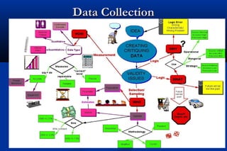
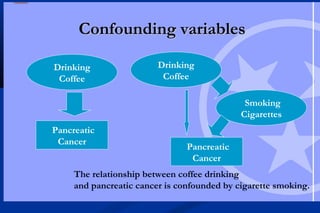
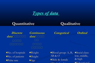
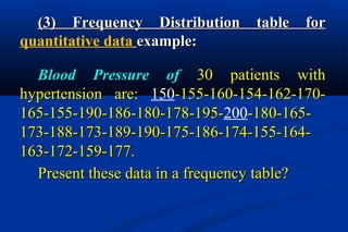
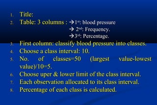
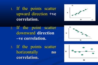
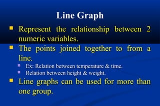
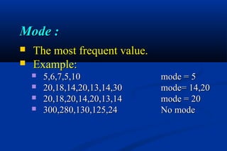
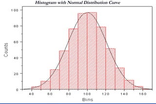
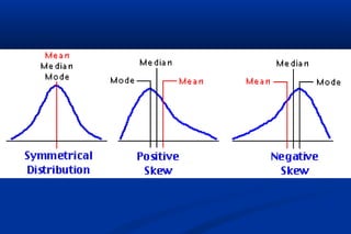
Statistics is the science of dealing with numbers and is used for collecting, summarizing, presenting, and analyzing data. It plays important roles in health care planning and evaluation, epidemiological studies, diagnosing community health problems, and comparing diseases and health status. Data can be quantitative or qualitative, discrete or continuous. Data is commonly presented using tables and graphs like bar charts, pie charts, histograms, scatter plots, and line graphs. Key measures used to summarize data include the mean, median, and mode for measures of central tendency, and the range, variance, and standard deviation for measures of dispersion.

1. STATISTICSSTATISTICS
Prof. Dr. Mona Aboserea

2. Definition:
Statistics is the science of dealing with numbers. It
is used for collection, summarization, presentation,
and analysis of data.
Uses:
 Planning & evaluation of health care programs.
Play a role in epidemiological studies.
Diagnosis of community health problems.
Comparison of diseases and health status.
Forming standards for biologic measurements e.g.
BP.
Differentiation between diseased and normal
groups.

3. 7-3
Data CollectionData Collection

4. Data : Observations made on
individuals.
Variable : any aspect of
individual that is measured e.g.
blood pressure, age.

6. Confounding variable: are two variables (explanatory
variables) that are confounded when their effects on a
response variable cannot be distinguished from each other

7. Confounding variablesConfounding variables
Drinking
Coffee
Pancreatic
Cancer
Drinking
Coffee
Smoking
Cigarettes
Pancreatic
Cancer
The relationship between coffee drinking
and pancreatic cancer is confounded by cigarette smoking.

8. Types of dataTypes of data
Quantitative Qualitative
DiscreteDiscrete
datadata‫تتتتتت‬‫تتتتتت‬
‫تتتت‬‫تتتت‬
‫تتتتتت‬‫تتتتتت‬
ContinuousContinuous
datadata‫تتتت‬‫تتتت‬
‫تت‬‫تت‬
‫تتتت‬‫تتتت‬
‫تتتتت‬‫تتتتت‬
CategoricalCategorical OrdinalOrdinal
No. of hospitalsNo. of hospitals
No. of patientsNo. of patients
Pulse ratePulse rate
WeightWeight
HeightHeight
AgeAge
Blood group: A, B,Blood group: A, B,
AB & OAB & O
Male & femaleMale & female
Social class:Social class:
low, middle,low, middle,
& high& high

10. Presentation of Data
Tabular Presentation .
Graphical Presentation .

11. I. Tabulation:I. Tabulation: criteria‫تتتت‬
‫تتتتتت‬
 Self explanatory.Self explanatory.
 Title at the top.Title at the top.
 Clear headings of columns and rows.Clear headings of columns and rows.
 Clear units of measurements.Clear units of measurements.
 Number of classes or rows from 2-10.Number of classes or rows from 2-10.
 2 types :2 types :  Listing tables.Listing tables.
 Frequency distribution table.Frequency distribution table.

12. No. of patients in each department at Zagazig hospitalNo. of patients in each department at Zagazig hospital
Department No. of patientsNo. of patients
Medicine
Surgery
ENT
Ophthalmology
100100
8080
4040
3030
Total 250250
(1) Listing table(1) Listing table

13. Distribution of students at public health lab 1
according to gender
Gender No. of studentsNo. of students
Male
Female
3535
2020
Total 5555
e.g. Listing tablee.g. Listing table

14. (2) Frequency distribution table for(2) Frequency distribution table for qualitativequalitative
data:data:
20 individuals of blood group: A- AB- AB-O-B-A-20 individuals of blood group: A- AB- AB-O-B-A-
A-B-B-AB-O-AB-AB-A-B-B-B-A-O-A.A-B-B-AB-O-AB-AB-A-B-B-B-A-O-A.
Distribution of the studied individuals according
to their blood group.
Blood group FrequencyFrequency %%
A
B
AB
O
66
66
55
33
3030
3030
2525
1515
TotalTotal 2020 100.00100.00

15. (3) Frequency Distribution table for(3) Frequency Distribution table for
quantitative data example:example:
Blood Pressure ofBlood Pressure of 30 patients with30 patients with
hypertension are:hypertension are: 150-155-160-154-162-170--155-160-154-162-170-
165-155-190-186-180-178-195-165-155-190-186-180-178-195-200-180-165--180-165-
173-188-173-189-190-175-186-174-155-164-173-188-173-189-190-175-186-174-155-164-
163-172-159-177.163-172-159-177.
Present these data in a frequency table?Present these data in a frequency table?

16. 1.1. Title:Title:
2.2. Table: 3 columns :Table: 3 columns : 11stst
: blood pressure: blood pressure
 22ndnd
: Frequency.: Frequency.
33rdrd
: Percentage.: Percentage.
3.3. First column: classify blood pressure into classes.First column: classify blood pressure into classes.
4.4. Choose a class interval: 10.Choose a class interval: 10.
5.5. No. of classes=50 (largest value-lowestNo. of classes=50 (largest value-lowest
value)/10=5.value)/10=5.
6.6. Choose uper & lower limit of the class interval.Choose uper & lower limit of the class interval.
7.7. Each observation allocated to its class interval.Each observation allocated to its class interval.
8.8. Percentage of each class is calculated.Percentage of each class is calculated.

17. Frequency Distribution of blood pressure
measurements among the studied group:
Blood PressureBlood Pressure
mmHgmmHg
FrequencyFrequency
%%
TallyTally No.No.
150-150-
160-160-
170-170-
180-180-
190-190-
200-200-
|||| ||||| |
|||| ||||| |
|||| ||||||| |||
|||| ||||| |
||||||
||
66
66
88
66
33
11
2020
2020
26.726.7
2020
1010
3.33.3
TotalTotal 3030 100.00100.00

19. II- Graphical Presentation
DefinitionDefinition::
Presenting data by using diagrams.Presenting data by using diagrams.
Graph should be :
Simple, understood.Simple, understood.
Save a lot of words.Save a lot of words.
Self explanatory.Self explanatory.
Clear title.Clear title.
Fully labeled.Fully labeled.
Vertical axis used for frequency.Vertical axis used for frequency.

20. Bar chart
 Used forUsed for discrete oror qualitativequalitative data.data.
 Data presented by rectangles separated byData presented by rectangles separated by
gaps,gaps, the length is proportional to the
frequency..
 Types of Bar charts:Types of Bar charts:
 Simple.Simple.
 Multiple.Multiple.
 ComponentComponent..

21. Simple bar chartSimple bar chart
Blood gp.Blood gp. Freq.Freq.
AA
BB
ABAB
OO
44
88
55
33
TotalTotal 2020
4
8
5
3
0
1
2
3
4
5
6
7
8
9
A B AB O
Blood Group
Frequency

22. 0%
10%
20%
30%
40%
50%
60%
70%
80%
90%
41%
47%
75%
5%
9.50%
2.90% 1.60%
58%
87.50%
risk factors
Associated risk factors for type 2 DM among
the studied patients

23. Multiple bar chartMultiple bar chart
Blood gp.Blood gp. Freq.Freq.
Female MaleFemale Male
AA
BB
ABAB
OO
33
66
77
44
44
88
55
33
TotalTotal 2020 2020
What is the defect in this char???????????

24. SE ClassSE Class %%
Egypt USAEgypt USA
LowLow
MiddleMiddle
HighHigh
6060
3030
1010
1010
6060
3030
TotalTotal 100100 100100
Component Bar Chart
FrequencyFrequency
%%
SE ClassSE ClassEgyptEgypt USAUSA
2020
4040
6060
8080
100100
What is the defect in this char???????????

25. Pie Chart
 Circle represent the total frequency
100%.
 Used in discrete or qualitative data.
 Divided into segments according to the
proportion of each category.
 2 pies can be used for comparison.

26. Disease %
Diarrhoea
Chest infection
Congenital
Accidents
50
30
10
10
Total 100
50%
30%
10%
10%

27. Gender Distribution of the studied patients
at diabetic center.
Female
Male

28. Histogram ::
 Used forUsed for quantitative continuous data.quantitative continuous data.
 Each class interval represented byEach class interval represented by
rectangle.rectangle.
 The height ofThe height of rectangle represent therepresent the
frequency.frequency.
 Rectangles areRectangles are adherent.

29. ht (cm)ht (cm) Freq.Freq.
100-100-
110-110-
120-120-
130-130-
140-140-
150-160150-160
1010
1414
2525
1717
1515
88
-100-100-110-110-120-120-130-130-140-140160 - 150160 - 150
Frequency

30. Frequency PolygonFrequency Polygon::
 Derived fromDerived from histogram..
 The midpoint of the rectangles’The midpoint of the rectangles’
top are connected.top are connected.
 It can be drawn withoutIt can be drawn without
histogram.histogram.

31. -100-100-110-110-120-120-130-130-140-140160 - 150160 - 150

32. 0
5
10
15
20
25
30
100-110-120-130-140-150-160

33. Scatter Diagram
 Used to represent the relationshipUsed to represent the relationship
betweenbetween 2 quantitative continuous
measurements.measurements.
 Each observation is represented by a pointEach observation is represented by a point
corresponding to its value on each axis.corresponding to its value on each axis.

34. 1.1. If the points scatterIf the points scatter
upward directionupward direction +ve
correlation.
2.2. If the point scatterIf the point scatter
downwarddownward direction
–ve correlation.
3.3. If the points scatterIf the points scatter
horizontallyhorizontally nono
correlation.correlation.

35. Line Graph
 Represent the relationship between 2Represent the relationship between 2
numeric variables.numeric variables.
 The points joined together to from aThe points joined together to from a
line.line.
 Ex: Relation between temperature & time.Ex: Relation between temperature & time.
 Relation between height & weight.Relation between height & weight.
 Line graphs can be used for more thanLine graphs can be used for more than
one group.one group.

36. Temperature
36
36.5
37
37.5
38
38.5
39
39.5
1 2 3 4 5 6 7
Time (hrs)Time (hrs)

37. 70
75
80
85
90
95
100
1 2 3 4
Time in days
HR
Drug 3Drug 3
Drug 2Drug 2
Drug 1Drug 1

38. Graphical Presentation
 Qualitative & discrete data:Qualitative & discrete data: * Bar Chart* Bar Chart
* Pie chart* Pie chart
 Quantitative continuous data:Quantitative continuous data:
 Histogram (e.g. population pyramid).Histogram (e.g. population pyramid).
 Frequency polygon (e.g. normal distribution curve)Frequency polygon (e.g. normal distribution curve)
 Relation between 2 numerical variables:Relation between 2 numerical variables:
 Scatter diagram.Scatter diagram.
 Line graph.Line graph.
Remember

40. While preparing the report of gastroenteritis
outbreak investigation the researcher wanted to
present the data i.e. number of cases related to
time, graphically. Which graph would you
suggest?
a) Bar chart
b) Pictogram
c) Pie chart
d) Histogram
e) Scatter diagram

42. Thank youThank you

43. Data SummarizationData Summarization
Measures ofMeasures of
central tendencycentral tendency
Measures ofMeasures of
dispersiondispersion
 Arithmetic meanArithmetic mean ..
 MedianMedian ..
 ModeMode ..
RangeRange
Variance.Variance.
Standard deviation.Standard deviation.
Coefficient ofCoefficient of
variation.variation.

44. I- Measures of central tendencyI- Measures of central tendency
 Describe the center of data:Describe the center of data:
X = meanX = mean  = sum= sum
X = value of observations.X = value of observations.
n= number of observations.n= number of observations.
1.1. Ungrouped data: 12, 15, 10, 17, 13.Ungrouped data: 12, 15, 10, 17, 13.
= 12+15+10+17+13/5 = 13.4= 12+15+10+17+13/5 = 13.4
n
X
X
∑=
n
X
X
∑=
n
X
X
∑=
n
X
X
∑=

45. 2. Grouped data without class interval:2. Grouped data without class interval:
Where f = frequency of each XWhere f = frequency of each X
n
X
X
∑=
n
X
X
∑=
n
fX
X
∑=
IP (days)(x)IP (days)(x) Freq. (f)Freq. (f) FxFx
22
33
44
55
66
22
44
11
33
22
44
1212
44
1515
1212
TT 12 (n)12 (n) 47 (47 (fx)fx)
X IP = 74/12 = 3.9 days.X IP = 74/12 = 3.9 days.

46. 3. Frequency data with class interval:3. Frequency data with class interval:
X1 = midpoint of class interval.X1 = midpoint of class interval.
n
X
X
∑=
n
X
X
∑=
Bl. PressureBl. Pressure
mmHg (x)mmHg (x)
Freq. (f)Freq. (f) Midpoint (xMidpoint (x11)) FxFx11
150-150-
160-160-
170-170-
180-180-
190-190-
200-210200-210
66
66
88
66
33
11
155155
165165
175175
185185
195195
205205
930930
990990
14001400
11101110
585585
205205
TT 30 (n)30 (n) 5220 (5220 (fxfx11))
* Mean blood pressure = 5220/30= 174 mmHg.* Mean blood pressure = 5220/30= 174 mmHg.
n
fX
X
∑=
1

47. (2) Median :(2) Median :
 Median is the middle observation in a series ofMedian is the middle observation in a series of
observations after arranging them in an assending orobservations after arranging them in an assending or
dessending manner.dessending manner.
1. If no. of observation is odds:1. If no. of observation is odds:
 A set of data 5,6,8,9,11A set of data 5,6,8,9,11 n=5n=5
 Median rank = n +1/2 = 5+1/2 = 3Median rank = n +1/2 = 5+1/2 = 3
 Median is the third value (8).Median is the third value (8).
2. If no. of observations is even:2. If no. of observations is even:
 A set of data 5,6,8,9A set of data 5,6,8,9 n=4n=4
 Median rank = 4+1/2= 5/2= 2.5.Median rank = 4+1/2= 5/2= 2.5.
 Median is the average of second & third value =Median is the average of second & third value =
6+8/2= 14/2= 7.6+8/2= 14/2= 7.

48. Mode :Mode :
 The most frequent value.The most frequent value.
 Example:Example:
 5,6,7,5,105,6,7,5,10 mode = 5mode = 5
 20,18,14,20,13,14,3020,18,14,20,13,14,30 mode= 14,20mode= 14,20
 20,18,20,14,20,13,1420,18,20,14,20,13,14 mode = 20mode = 20
 300,280,130,125,24300,280,130,125,24 No modeNo mode

49. II- Measures of dispersion:II- Measures of dispersion:
 Describe the degree of variation of dataDescribe the degree of variation of data
around the central values:around the central values:
1. Range = largest observation – smallest observation.1. Range = largest observation – smallest observation.
(mean-x)(mean-x)22
2. Variance (V) = ----------------------2. Variance (V) = ----------------------
n – 1n – 1
n
X
X
∑=
n
X
X
∑=

50. 3. Standard deviation (SD):3. Standard deviation (SD):
(X-X)(X-X)22
SD = V = -------------SD = V = -------------
n-1n-1
4. Coefficient of variation (CV)4. Coefficient of variation (CV)
The percentage of SD from the meanThe percentage of SD from the mean
CV = SD/mean x 100CV = SD/mean x 100
n
X
X
∑=
n
X
X
∑=

51. ExampleExample
1. Set of observation 5, 7, 10, 12, 161. Set of observation 5, 7, 10, 12, 16
X = 5+7+10+12+16/5 = 50/5 = 10X = 5+7+10+12+16/5 = 50/5 = 10
(10-5)(10-5)22
++ (10-7)(10-7)22
+(10-10)+(10-10)22
+(10-12)+(10-12)22
+(10-16)+(10-16)22
7474
SD= -------------------------------------------------------- = ------- = 4.3SD= -------------------------------------------------------- = ------- = 4.3
5 – 15 – 1 44
CV = 4.3/10 x 100 = 43%CV = 4.3/10 x 100 = 43%
2. Set of observations 2, 2, 5,10, 112. Set of observations 2, 2, 5,10, 11
X = 2+2+5+10+11/5 = 30/5 = 6X = 2+2+5+10+11/5 = 30/5 = 6
(6-2)(6-2)22
+(6-2)+(6-2)22
+(6-5)+(6-5)22
+(6-10)+(6-10)22
+(6-11)+(6-11)22
7474
SD= -------------------------------------------------------- = ------- = 4.3SD= -------------------------------------------------------- = ------- = 4.3
5 – 15 – 1 44
CV = 4.3/6 x 100 = 71.6%CV = 4.3/6 x 100 = 71.6%

52. Histogram with Normal Distribution Curve

53. Frequency polygon with Normal Distribution Curve

54. Normal Distribution CurveNormal Distribution Curve
(Guassian Curve)(Guassian Curve)
 A frequency polygon used in presentationA frequency polygon used in presentation
continuous quantitative variables as age,continuous quantitative variables as age,
weight, height, Hb level, bl. pressure.weight, height, Hb level, bl. pressure.
 Normal distribution curve is used to identifyNormal distribution curve is used to identify
normal & abnormal measurements.normal & abnormal measurements.

55. Characteristics of the CurveCharacteristics of the Curve
 Bell-shaped, continuous.Bell-shaped, continuous.
 Symmetrical.Symmetrical.
 The tail extend to infinity.The tail extend to infinity.
 Mean, mode, median coincide.Mean, mode, median coincide.
 Described by:Described by: - arithmatic means ( )- arithmatic means ( )
- standard deviation (SD)- standard deviation (SD)
 Area under the normal curve:Area under the normal curve:
± 1 SD = 68%± 1 SD = 68%
± 2 SD = 95%± 2 SD = 95%  the normal rangethe normal range
± 3 SD = 99%± 3 SD = 99%
X
X
X
X

57. Distribution of DataDistribution of Data

59. Example:Example:
 In normal distribution curve for blood HbIn normal distribution curve for blood Hb
level for normal adult ♂:level for normal adult ♂:
Mean = 11Mean = 11 SD= ± 1.5SD= ± 1.5
 Hb of an individual is 8.1 is he normal orHb of an individual is 8.1 is he normal or
anaemic?anaemic?
 The higher level of Hb = 11+2 x 1.5 = 14The higher level of Hb = 11+2 x 1.5 = 14
 The lower level of Hb = 11- 2 x 1.5 = 8The lower level of Hb = 11- 2 x 1.5 = 8
 The normal range of Hb in adult ♂ is 8-14The normal range of Hb in adult ♂ is 8-14
 Our patient (8.1) is normal.Our patient (8.1) is normal.

60. Thank youThank you

61. Inferential Statistics
Prof. Dr. Mona Aboserea

62. N.B.N.B. Research ProcessResearch Process
Research question
Hypothesis
Identify research design
Data collection
Presentation of data
Data analysis
Interpretation of data

63. What is a Statistic????
Population
Sample
Sample
Sample
Sample
Parameter: value that describes a population
Statistic: a value that describes a sample
 always using samples!!!

64. Statistics
Descriptive Statistics
• Organize
• Summarize
• Simplify
• Presentation of data
Inferential Statistics
•Generalize from
samples to pops
•Hypothesis testing
•Relationships among
variables
Describing data
Make predictionsMake predictions

65. Inferential Statistics
.

66. Inferential StatisticsInferential Statistics
 Inferential statistics are used to draw conclusions
about a population by examining the sample
POPULATION
Sample

67. Sample
Inference
Population

68.  Inference:Inference: making a generalization about amaking a generalization about a
larger group of population on the basis of alarger group of population on the basis of a
sample.sample.
 Inferential statistics Instead of using the
entire population to gather the data, the
statistician will collect a sample or samples
from the millions of residents and make
inferences about the entire population using
the sample.

69.  Hypothesis (significance) testing:Hypothesis (significance) testing:
Conducting of significance test to find outConducting of significance test to find out
whether the observed variation among sampling iswhether the observed variation among sampling is
due todue to chance or it is a really difference.chance or it is a really difference.

70. General principles (steps) of
significance tests
 Set up the null hypothesis & its alternative.Set up the null hypothesis & its alternative.
 Set level of significance:Set level of significance:
In medicine, we consider the difference are significantIn medicine, we consider the difference are significant
if the probability (P value) is less thanif the probability (P value) is less than 0.05.
 Find theFind the value of the test statistics (calculatedvalue of the test statistics (calculated
value)value)..

71. General principles (steps) of
significance tests
 Find the tabulated value.Find the tabulated value.
 Conclude that the data are consistent orConclude that the data are consistent or
inconsistent with theinconsistent with the null hypothesis byby
comparing the two values. If data are notcomparing the two values. If data are not
consistent with null hypothesis we rejectconsistent with null hypothesis we reject
it & the difference isit & the difference is statistically
significant & the vice versa.& the vice versa.

73. Null & alternative hypothesis
For quantitative data
 In null hypothesis (H0): X1=X2 or X1-X2=0.
 Alternative hypothesis (H1) is postulated
(Research hypothesis).
H1 : X1<X2 or H1: X2<X1. or X1 ≠ X2
or X1-X2 ≠ 0

74. N.B. Statistics demonstrate association, but not
causation
H0: There is no association between the
exposure and disease of interest
H1: There is an association between the
exposure and disease of interest
74
Hypothesis Testing
For qualitative data

75. Chain of Reasoning for
Inferential Statistics
Population
Sample
Inference
Selection
Measure
Probability
data
Are our inferences valid?…Best we can do is to calculate probability
about inferences

76. Inferential Statistics: uses sample data to evaluate the
credibility of a hypothesis about a population
NULL Hypothesis:
NULL (nullus - latin): “not any”  no
differences between means
H0 : m1 = m2
“H- Naught”Always testing the null hypothesis

77. Inferential statistics: uses sample data to evaluate the
credibility of a hypothesis about a population
Hypothesis: Scientific or alternative
hypothesis
Predicts that there are differences between the groups
H1 : m1 = m2

78. Hypothesis
A statement about what findings are expected
null hypothesis
"the two groups will not differ“
alternative hypothesis
"group A will do better than group B"
"group A and B will not perform the same"

79. Inferential Statistics
When making comparisons
btw 2 sample means there are 2
possibilities
Null hypothesis is true
Null hypothesis is false
Not reject the Null Hypothesis
Reject the Null hypothesis
Statistical significanceNo Statistical significance

80. D+
D-
E+
15 85
E-
10 90
Example:
IE+ = 15 / (15 + 85) = 0.15
IE- = 10 / (10 + 90) = 0.10
RR = IE+/IE- = 1.5, p value = 0.30
Although it appears that the incidence of disease may be
higher in the exposed than in the non-exposed (RR=1.5),
the p-value of 0.30 exceeds the fixed alpha level of 0.05.
This means that the observed data are relatively
compatible with the null hypothesis. Thus, we do not
reject H0 in favor of H1 (alternative hypothesis).

81. 2.5% 2.5%
5% region of rejection of null hypothesis
Non directional
Two Tail

82. 5%
5% region of rejection of null hypothesis
Directional
One Tail

83. N.B.N.B. In medicineIn medicine
We consider that differences are significant
if the probability (p value) is less than 0.05
this means that:
 if the null hypothesis is true, we will make aif the null hypothesis is true, we will make a
wrong decision less than 5 in a hundredwrong decision less than 5 in a hundred
times.times.

84. Hypothesis Testing Flow ChartHypothesis Testing Flow Chart
Develop research hypothesis H1 & null hypothesis H0
Set significance level (usually .05(
Collect data
Calculate test statistic and p value
Compare p value to
alpha (.05(
P < .05 P > .05
Reject null hypothesis Fail to reject null hypothesis
Statistical significance No Statistical significance

85. Tests of significance
are methods to assess the hypothesis
testing

86. Matched
Groups
Paired t test

87. ((A) Quantitative dataA) Quantitative data
1.1. Compare 2 means of large sample (≥60) & followCompare 2 means of large sample (≥60) & follow
normal distributionnormal distribution 
Z testZ test (SND)(SND) ==
(population mean – sample mean)/SD(population mean – sample mean)/SD

88. If the result of Z >2 then there is significant difference.
As we mentioned before the normal range for any
biological reading lies between the mean value of the
population reading ± 2 SD.
(this range includes 95% of the area under the normal
distribution curve).

89. 2. Compare 2 means of small sample (<60)2. Compare 2 means of small sample (<60) 
 tt test =test = df=ndf=n11+n+n22 -2-2

The value ofThe value of tt is compared to the values inis compared to the values in
t-tablet-table at the value of degree of freedom.at the value of degree of freedom.
2
2
2
1
2
1
21
n
SD
n
SD
xx
+
−

90.  TheThe value of tvalue of t will be compared to values in thewill be compared to values in the
specific table ofspecific table of "t distribution test""t distribution test" at theat the
value of the degree of freedom.value of the degree of freedom.

If the value ofIf the value of tt isis less thanless than that in the table,that in the table,
then the difference between samples isthen the difference between samples is
insignificant.insignificant.
 If theIf the t valuet value isis larger thanlarger than that in the table sothat in the table so
the difference is significant i.e.the difference is significant i.e. the nullthe null
hypothesis is rejected (significant).hypothesis is rejected (significant).

91. Serum cholesterol levels for two groups of EgyptiansSerum cholesterol levels for two groups of Egyptians
were recorded. The mean cholesterol levels of thewere recorded. The mean cholesterol levels of the
two groups were compared. To determine whethertwo groups were compared. To determine whether
the measurements were significantly different or not,the measurements were significantly different or not,
the most appropriate statistical test would be:the most appropriate statistical test would be:
a. Chi-square testa. Chi-square test
b. Correlation analysisb. Correlation analysis
c. F test (ANOVA)c. F test (ANOVA)
d. Student’s t testd. Student’s t test
e. Regression analysise. Regression analysis

92. In a study carried out to assess the hemoglobin level of two groupsIn a study carried out to assess the hemoglobin level of two groups
of students, one group of them was suffering from parasiticof students, one group of them was suffering from parasitic
infestation.infestation.
The following was found out:The following was found out:
Group1
Healthy
)Hb level(
Group2 parasitic
infestation
)Hb level(
12 10
13 9
16 12
13 11
15 8
16 10.5
15 11
14 9.5
14 13
11 11
Is there a statistical significant
difference between the two
groups?
)P value < 0.05 if test results
> 2.11 (
Tabulated value

95. AnswerAnswer

96. 3-Paired t test:3-Paired t test:
 Compare Means of twoCompare Means of two matched samplesmatched samples oror
means of repeated observation in the samemeans of repeated observation in the same
individualindividual )Pre & post()Pre & post(..
 Paired t-test =the mean difference divided byPaired t-test =the mean difference divided by
)standard deviation difference between each pair ∕)standard deviation difference between each pair ∕
√√n(n(

97. Six volunteers took a cholesterol lowering diet for 3Six volunteers took a cholesterol lowering diet for 3
months and mean cholesterol levels were measuredmonths and mean cholesterol levels were measured
beforebefore andand afterafter the trial diet. The appropriate test ofthe trial diet. The appropriate test of
statistical significance for this trial will be:statistical significance for this trial will be:
a) Chi-square testa) Chi-square test
b) Odd’s ratiob) Odd’s ratio
c) Paired t- testc) Paired t- test
d) Student t-testd) Student t-test
e) Z tesTe) Z tesT

98. 4-Analysis of variance )ANOVA = F test(:
Comparing several means:
D-F = (d.f between groups, df within groups)D-F = (d.f between groups, df within groups)
= K – 1, N – K= K – 1, N – K
Mean square difference between groups
F= Mean square difference within groups

99.  A-One way analysis of variance:A-One way analysis of variance: It is used toIt is used to
compare means of more than 2 groups by a definedcompare means of more than 2 groups by a defined
one factorone factor e.g.e.g. )BG in 3 groups of pts: 1-lifestyle,)BG in 3 groups of pts: 1-lifestyle,
2-OHA, 3-Insulin therapy(2-OHA, 3-Insulin therapy(

100. e.g. Comparing mean blood glucose levels amonge.g. Comparing mean blood glucose levels among
the studied groups of T2diabetic patientsthe studied groups of T2diabetic patients
Variable Life style
group
)diet +exercise(
Mean +SD
Oral
hypoglycemic
drugs
Mean +SD
Insulin
therapy
group
Mean +SD
ANOVA
&
P value
Random
Blood
glucose
(mg/dl)
135+45.5 127+42.5 118.5+25.5

101.  B- Two – way analysis of variance:B- Two – way analysis of variance: is used tois used to
compare the means of more than 2 groups bycompare the means of more than 2 groups by
more than one factormore than one factor e.g.e.g. )BG & cholesterol)BG & cholesterol
level in 3 groups of pts: 1-lifestyle, 2-OHA,level in 3 groups of pts: 1-lifestyle, 2-OHA,
3-Insulin therapy(3-Insulin therapy(

102. e.g. Comparing mean blood glucose &e.g. Comparing mean blood glucose &
cholesterol levels among the studied groups ofcholesterol levels among the studied groups of
T2diabetic patientsT2diabetic patients
Variable Life style
group
)diet
+exercise(
Mean
+SD
Oral
hypoglyce
mic drugs
Mean
+SD
Insulin
therapy
group
Mean +SD
ANOVA
&
P value
Random
Blood
glucose
(mg/dl)
135+45.5 127+42.5 118.5+25.5
Cholester
ol level
180 + 67 179 + 77.5 174 + 66.4

104. )B( Qualitative Variables
1. Chi = square test (x1. Chi = square test (x22
):):
== df= (row-1)(column-1)df= (row-1)(column-1)
 O = observed valueO = observed value
 E= expected value =E= expected value =
==
∑
−
E
EO 2
)(
totalgrand
totalcolumnxtotalrow
2
χ

105. Association between physical activity andAssociation between physical activity and
weightweight
Obese-
overwt
Average wt Total
Lack of
activity
70 (E1) 30 (E2) 100
Physical
activity
10 (E3) 90 (E4) 100
Total 80 120 200
N.B. Chi-square value at DF=1 equal 3.8

106. XX22‌‌‌‌‌‌‌‌
==
)70-40()70-40(22
∕40∕40 ++ )30-60()30-60(22
∕60∕60++)10-40()10-40(22
∕40∕40 ++ )90-60()90-60(22
∕60=∕60=
22.5 + 15 + 22.5 +15=22.5 + 15 + 22.5 +15= 7575
calculated value > tabulated valuecalculated value > tabulated value
p=0.0000p=0.0000
Obese-
overwt
Average wt Total
Lack of
activity
70 (40) 30 (60) 100
Physical
activity
10 (40) 90 (60) 100
Total 80 120 200

107. Example:Example:
The result of influenza vaccine trial.The result of influenza vaccine trial.
InfluenzaInfluenza
VaccineVaccine
O EO E
PlaceboPlacebo
O EO E
TT
YesYes
NoNo
6060
4040
4040
6060
100100
100100
100100 100100 200200
 Expected value in every cell =Expected value in every cell =
R total x C totalR total x C total
= --------------------------= --------------------------
G totalG total

108.  ==
==
∑
−
E
EO 2
)(2
χ

111. (2) Z- test(2) Z- test to compare 2 proportions:to compare 2 proportions:
ZZ ==
 PP11= % of first group.= % of first group.
 PP22=% of second group.=% of second group.
 qq11= 100-p= 100-p1.1.
 qq22=100-p=100-p2.2.
 nn11=size of first group.=size of first group.
 nn22=size of second group.=size of second group.
 IfIf Z>2Z>2, the difference is statistically significance., the difference is statistically significance.
2
22
1
11
21
n
qp
n
qp
PP
+
−

112. Example:Example:
 No of anaemic patients in group 1(50) is 5.No of anaemic patients in group 1(50) is 5.
 No of anaemic patients in group 2(60) is 20.No of anaemic patients in group 2(60) is 20.
 Find if gp 1 & 2 are statistically different inFind if gp 1 & 2 are statistically different in
the prevalence of anaemia.the prevalence of anaemia.
 We use Z test:We use Z test:
PP11= 5/50 x 100= 10%.= 5/50 x 100= 10%. PP22=20/60 x 100 = 33%.=20/60 x 100 = 33%.
qq11= 100-10= 90% .= 100-10= 90% . qq22=100-33= 67.=100-33= 67.
nn11=50.=50. nn22=60.=60.

113. Z =Z =
 Z = 3.1 > 2 so, there is statisticallyZ = 3.1 > 2 so, there is statistically
significant difference between thesignificant difference between the
precentages of anaemia between the 2precentages of anaemia between the 2
groups.groups.
1.34.7/23
85.3618
23
60
6733
50
9010
3310
==
+
=
+
−
xx

114. Correlation & Regression
 Correlation: measure the degree of associationmeasure the degree of association
between 2 continuous variables.between 2 continuous variables.
 Correlation is measured byCorrelation is measured by correlationcorrelation
coefficientcoefficient (r)(r)..
 Value of r ranged betweenValue of r ranged between +1 & -1.+1 & -1.
 r=0 means no correlation.r=0 means no correlation.
 r=+1 means perfect +ve association.r=+1 means perfect +ve association.
 r=-1 means perfect -ve association.r=-1 means perfect -ve association.
 t-testt-test for correlation is used to test thefor correlation is used to test the
significance of association.significance of association.

115. Pearson correlationPearson correlation
(r(r((

116. Scatter PlotsScatter Plots
Strong Negative Correlation
X
Y
r = -0.86
Strong Positive Correlation
X
Y
r = 0.91
Positive Correlation
X
Y
r = 0.70
No Correlation
X
Y
r = 0.06

117. Variable Pearson
correlation
)r(
P value
MCV, fl 0.94 0.000*
Platelet counts X 109
-0.42 0.061
Ferritin 0.61 0.081
Table ) (: Correlation between hemoglobin level
and MCV, platelet counts, and Ferritin
among the studied cases.

118. Correlation and regressionCorrelation and regression

119.  RegressionRegression gives equation for the line that bestgives equation for the line that best
models the relationship between 2 variables.models the relationship between 2 variables.
 Types of patternTypes of pattern:: linear, curve,linear, curve, …. Will determine…. Will determine
the type of regression model to be applied to the data.the type of regression model to be applied to the data.
 Linear regressionLinear regression: is the simplest form & is used: is the simplest form & is used
when the relation between x & y variables iswhen the relation between x & y variables is
approximated by straight line.approximated by straight line.
 Linear regressionLinear regression gives thegives the equation of the straightequation of the straight
line that determine the relation an prediction of aline that determine the relation an prediction of a
change in a variable )dependant( due to change inchange in a variable )dependant( due to change in
the other variable )independentthe other variable )independent).).

120. Linear diagramLinear diagram

121.  t-testt-test is used to assess the level ofis used to assess the level of
significance.significance.
 Multiple regressionMultiple regression : used to assess the: used to assess the
dependency of a dependant variable ondependency of a dependant variable on
several independent variables.several independent variables.
 F-testF-test (ANOVA) is the test of(ANOVA) is the test of
significance.significance.
e.g.e.g. vit D levelvit D level ((age, amount of ca intake,age, amount of ca intake,
duration of exposure to sunduration of exposure to sun, ……), ……)

122. Thank youThank you