Downloaded 225 times


This document provides an overview of key concepts in biostatistics. It defines biostatistics as the application of statistical methods in the fields of biology, public health, and medicine. Some key points covered include: - The types of data: qualitative, quantitative, discrete, continuous - Descriptive statistics like mean, median, and mode - Inferential statistics like hypothesis testing and estimating parameters - Important statistical tests like t-tests, ANOVA, and chi-squared tests - Measures of diagnostic accuracy like sensitivity, specificity, and predictive values - The process of determining sample size for studies based on factors like confidence interval, power, and allowable error.
Introduction slide with presenter information.
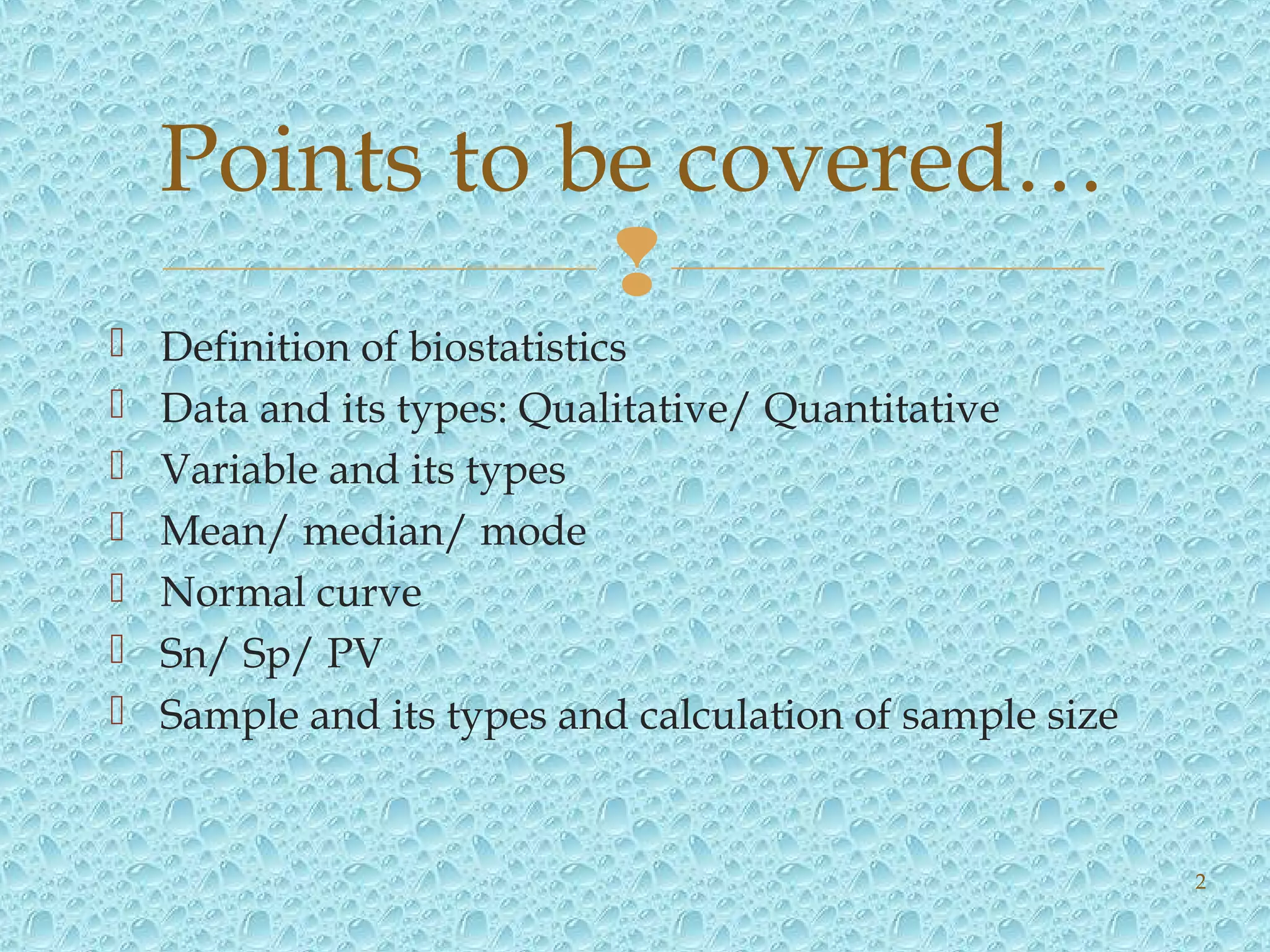
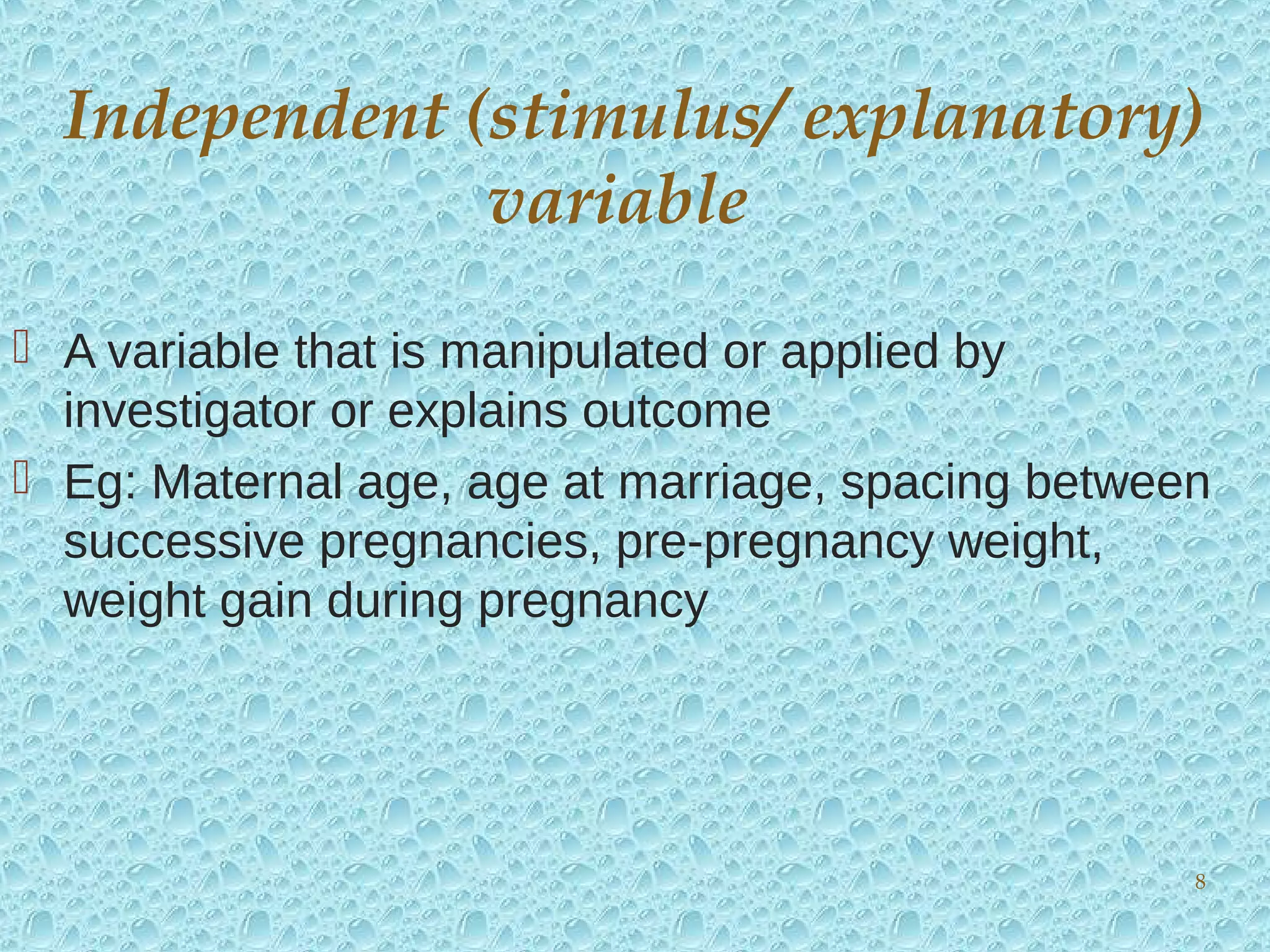
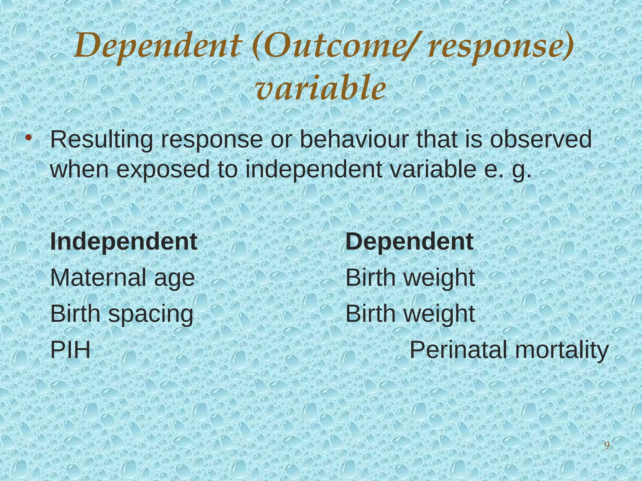
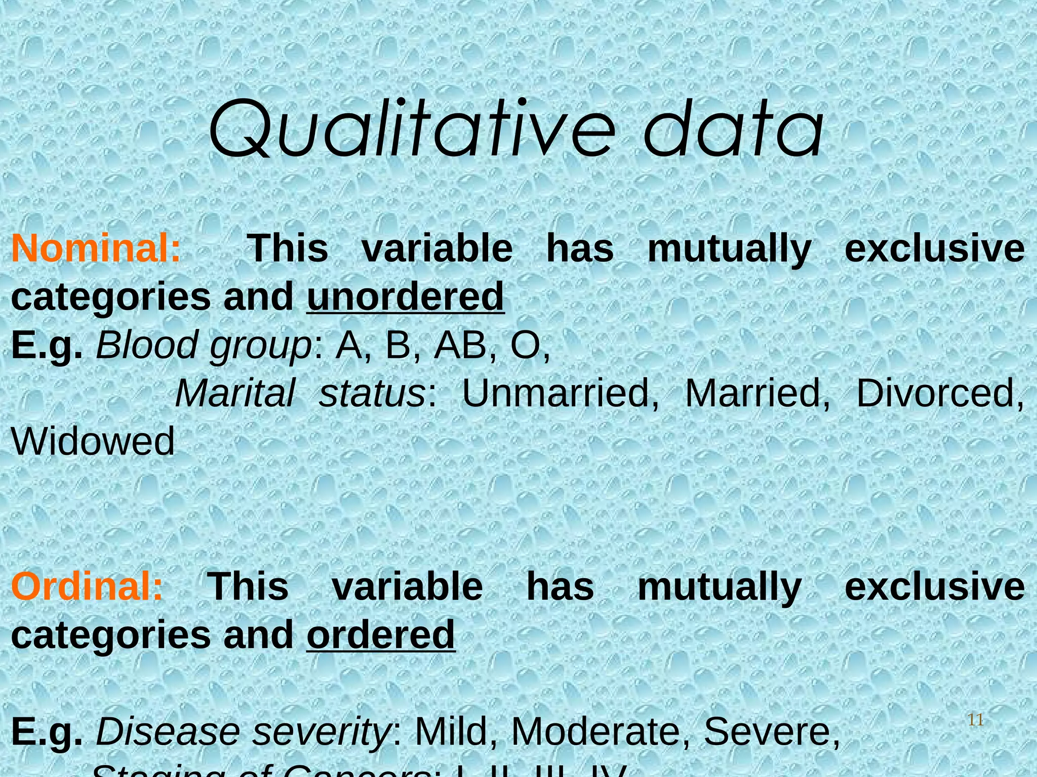
Definitions, types of data, variables, and the importance of statistics in medicine and public health.
Primary vs Secondary data, variables, and significance of qualitative and quantitative data.
Descriptive statistics summarizing data and inferential statistics for hypothesis testing.
Point and interval estimates, including confidence intervals, and steps in hypothesis testing.
Null and alternative hypotheses, basic terms related to hypothesis testing.
Discussion on parametric tests, normal distribution, and its properties.
Detailed features and significance of the normal distribution in data analysis.
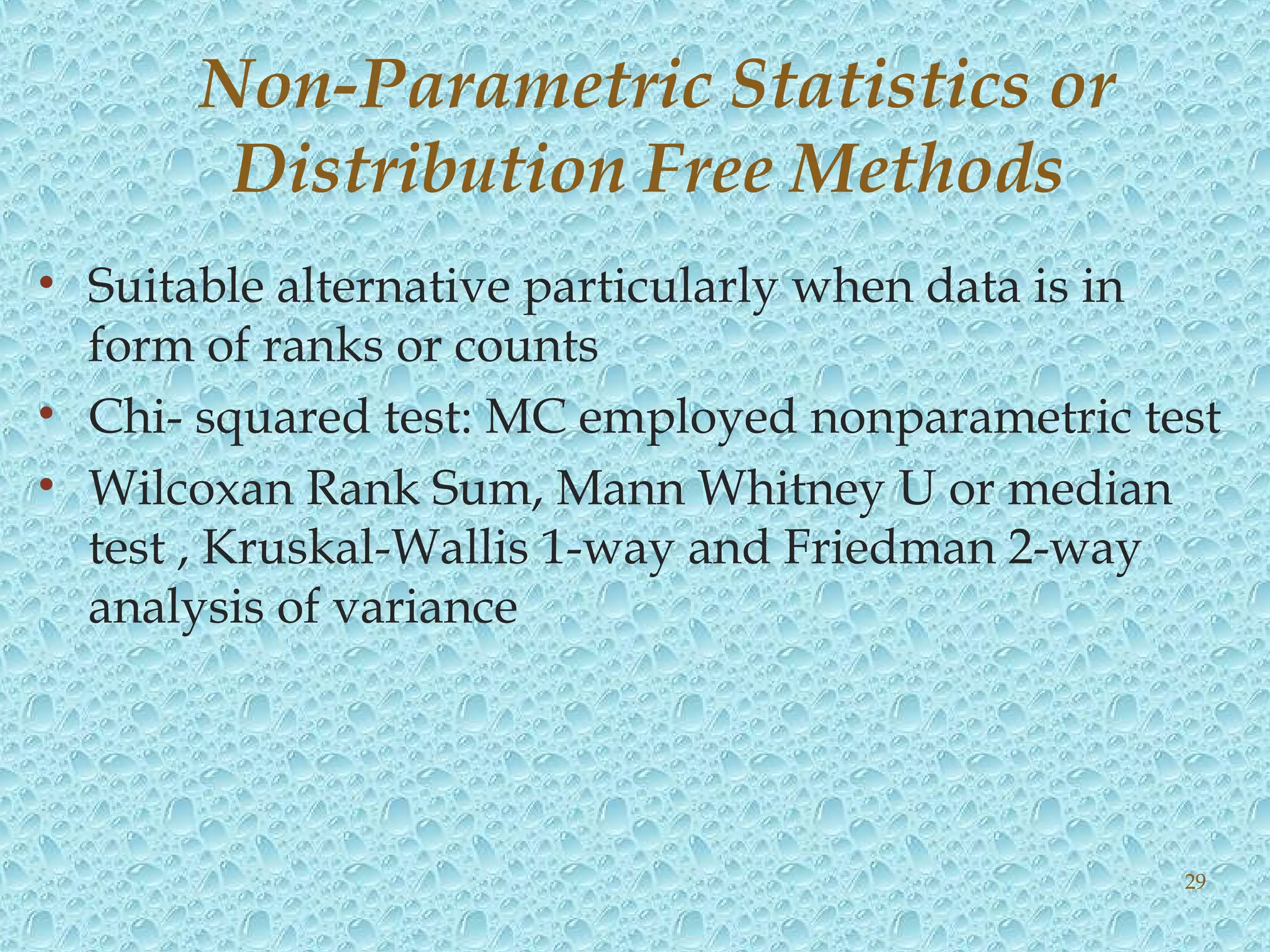
Explanation of skewed data and the usage of non-parametric statistics.
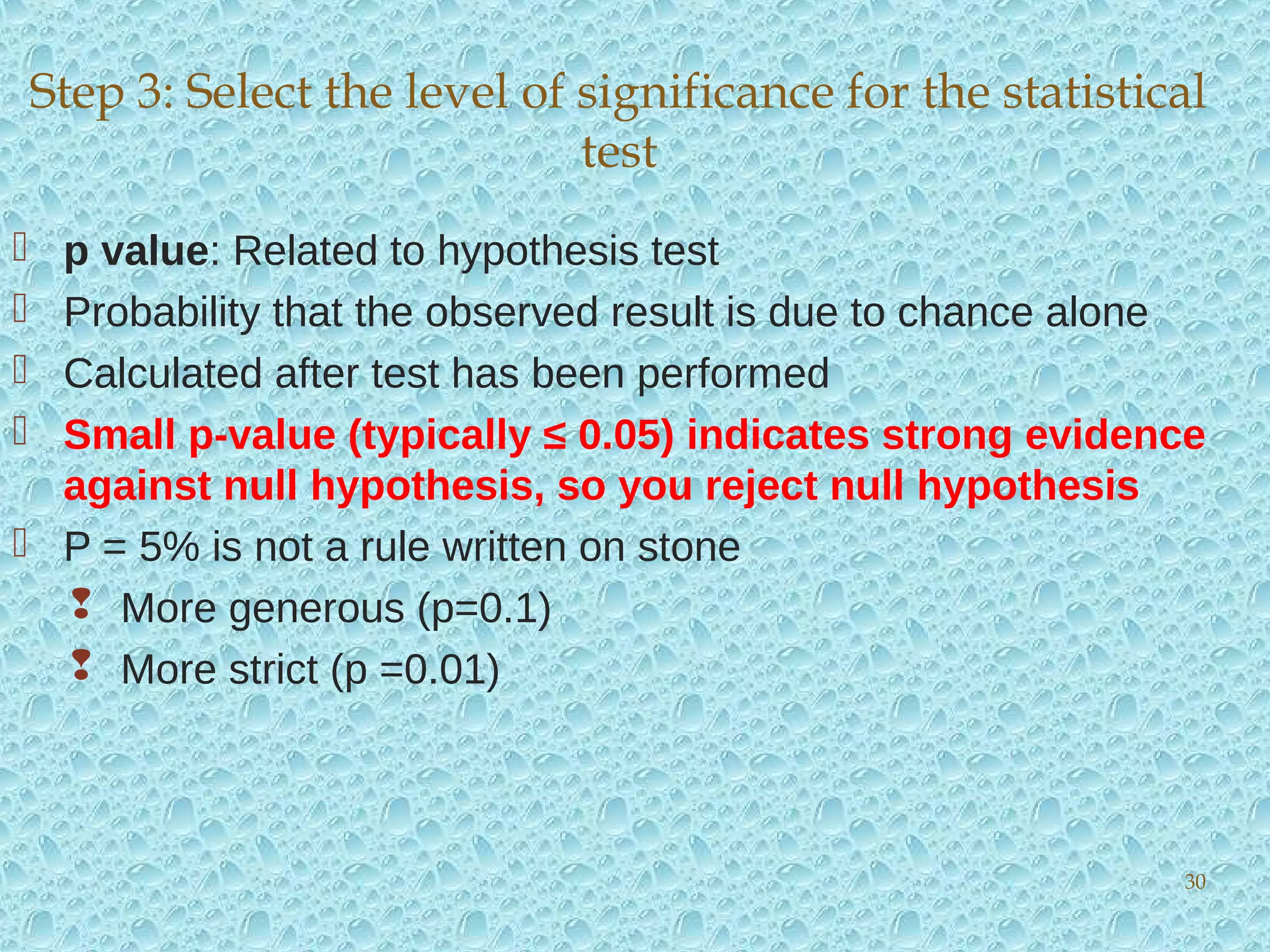
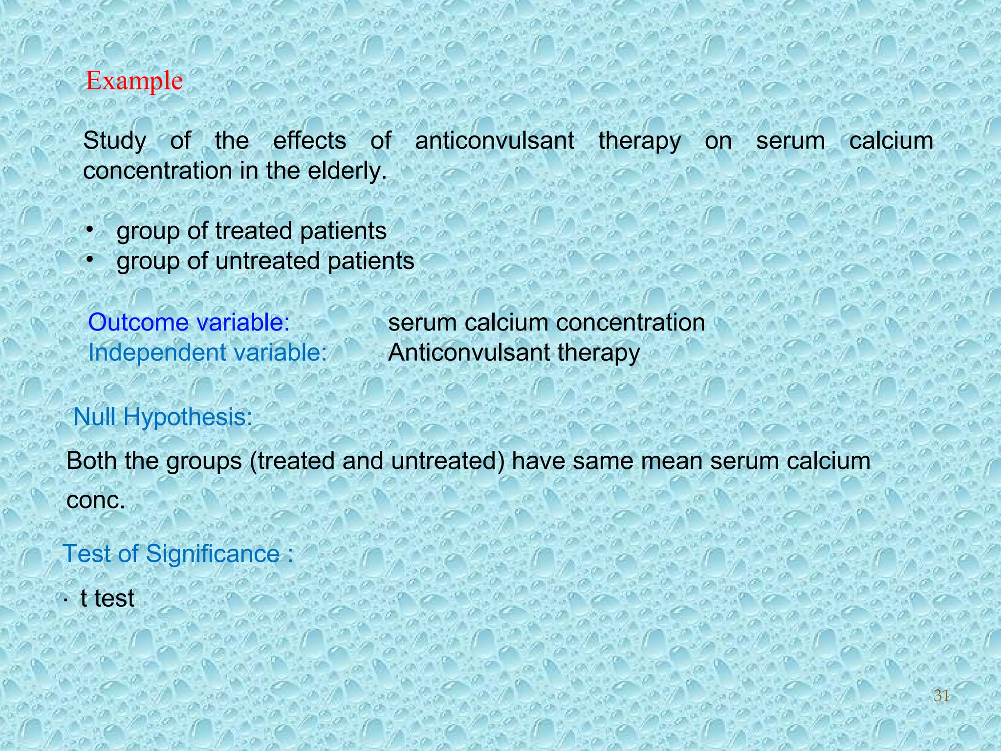
Understanding p-values in hypothesis testing with an example study.
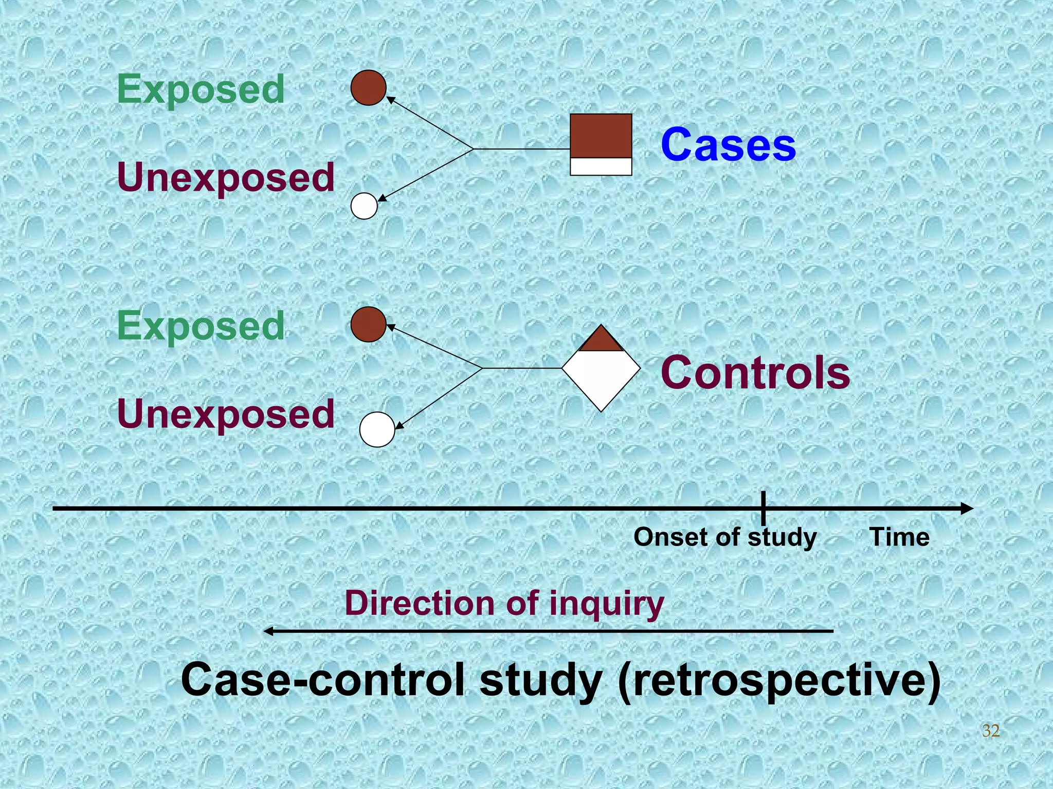
Case-control study methodologies and explanation of odds ratios and relative risk.
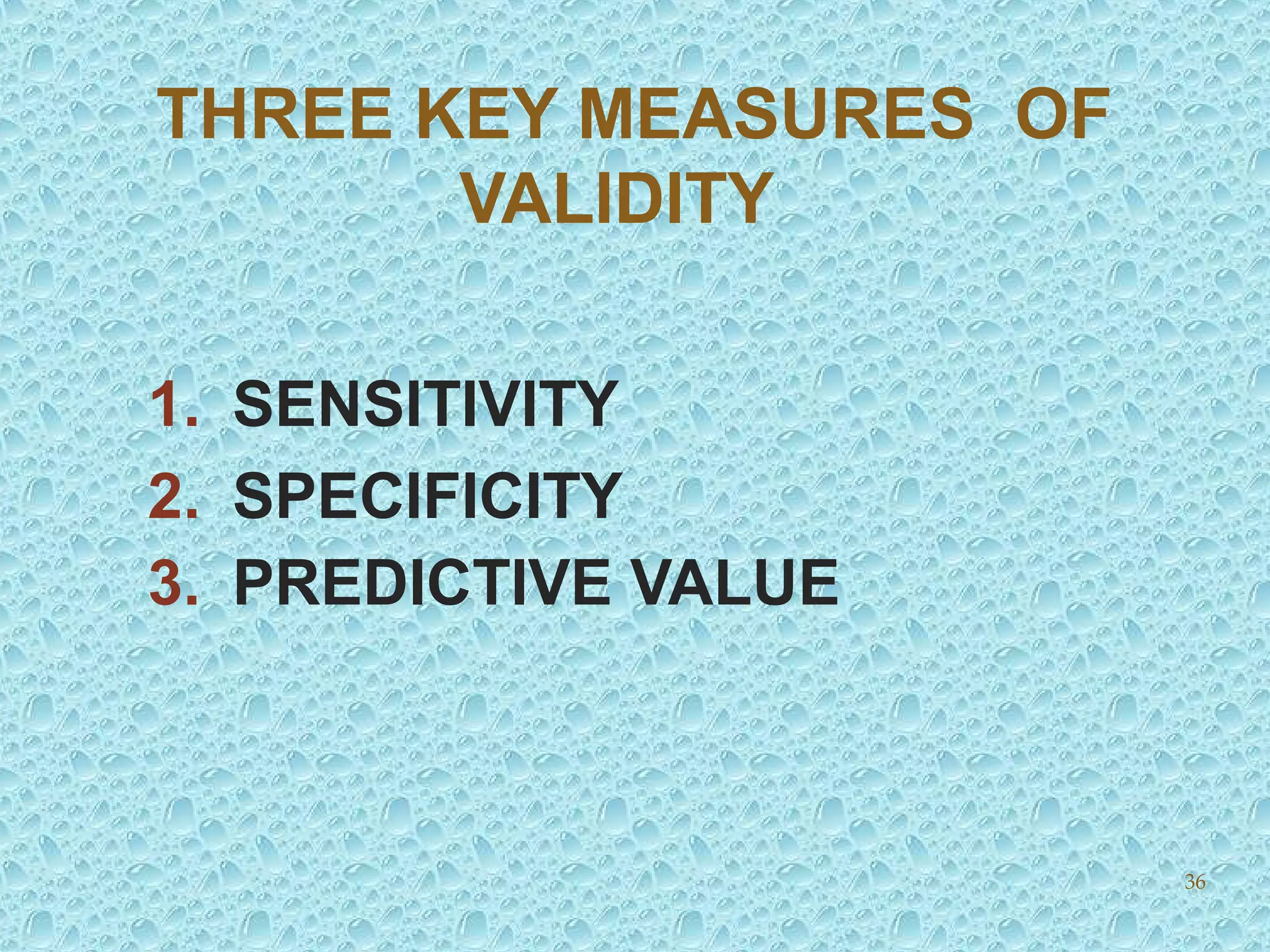
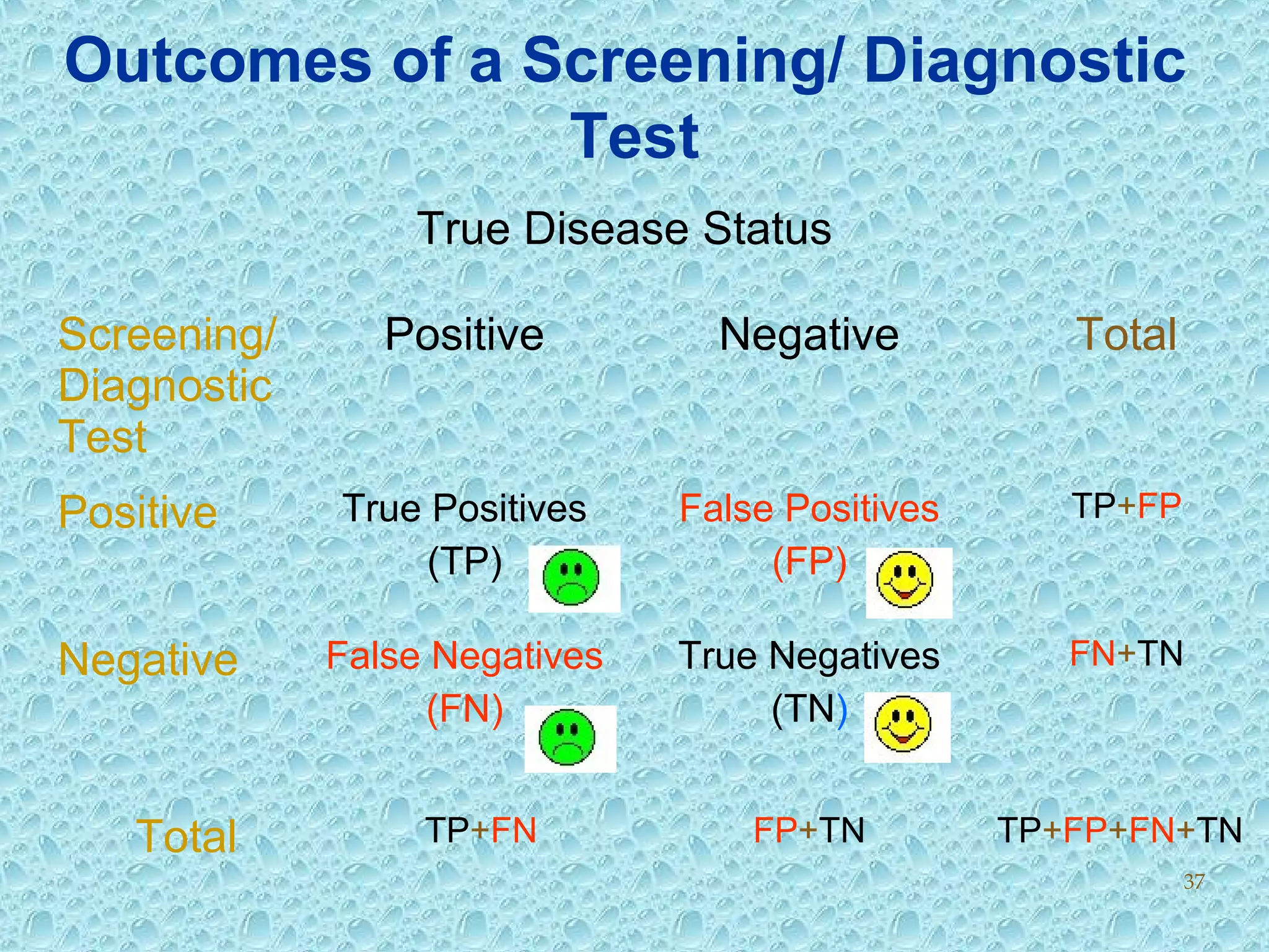
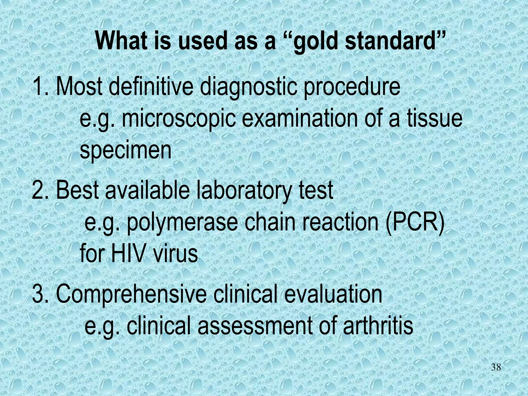
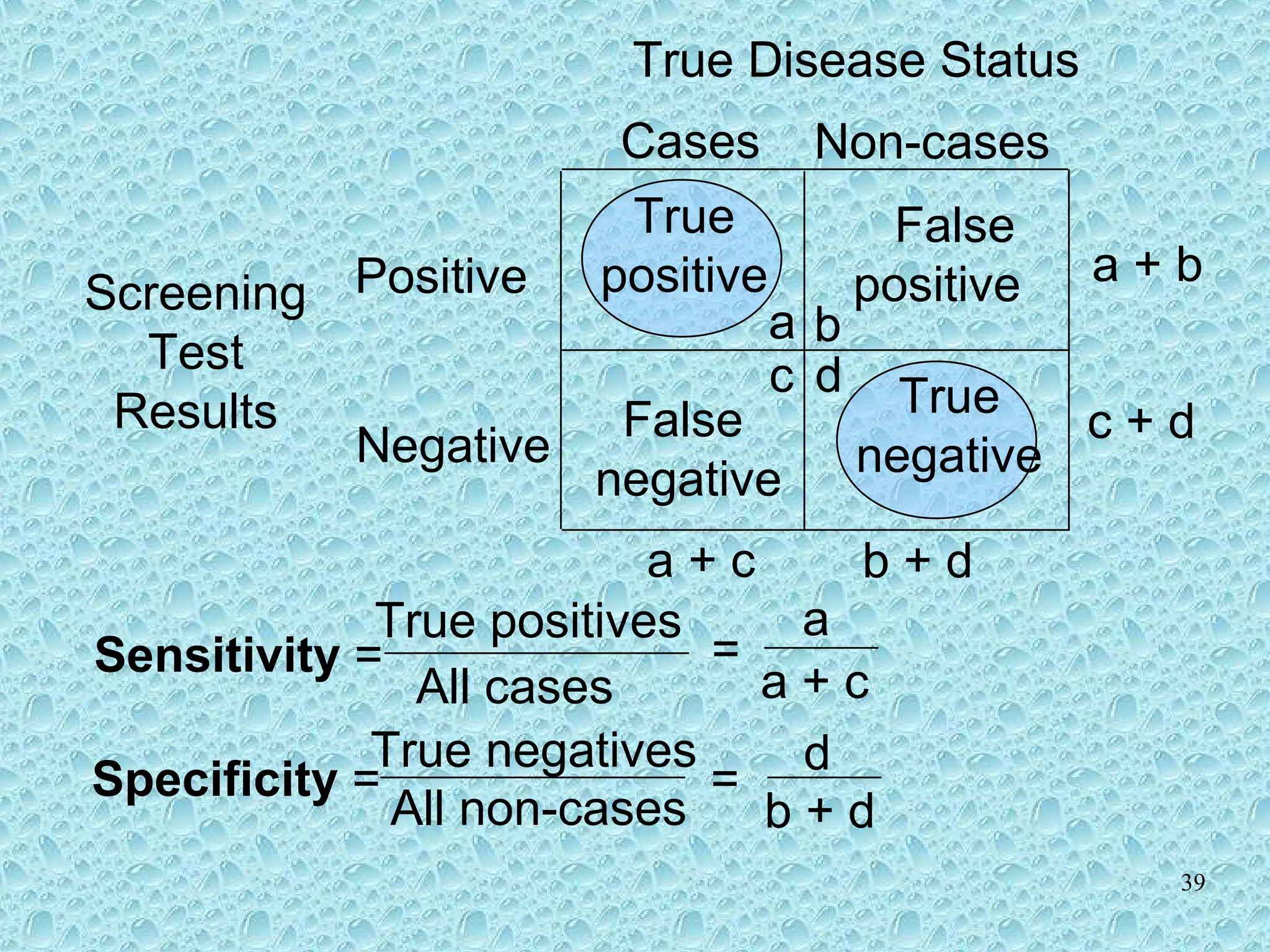
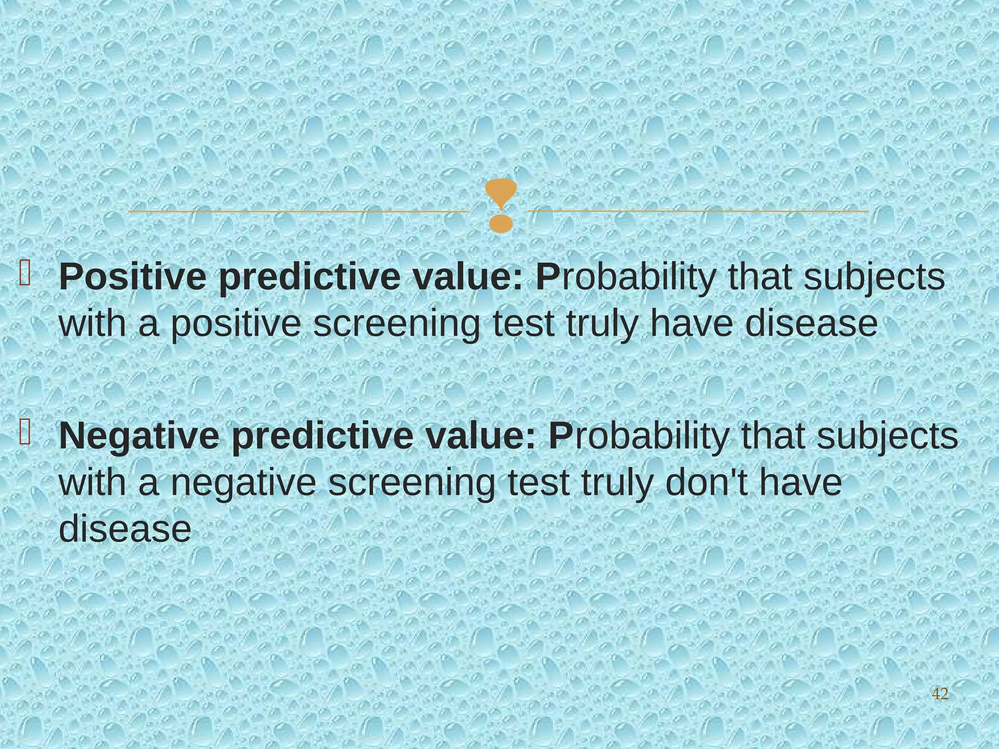
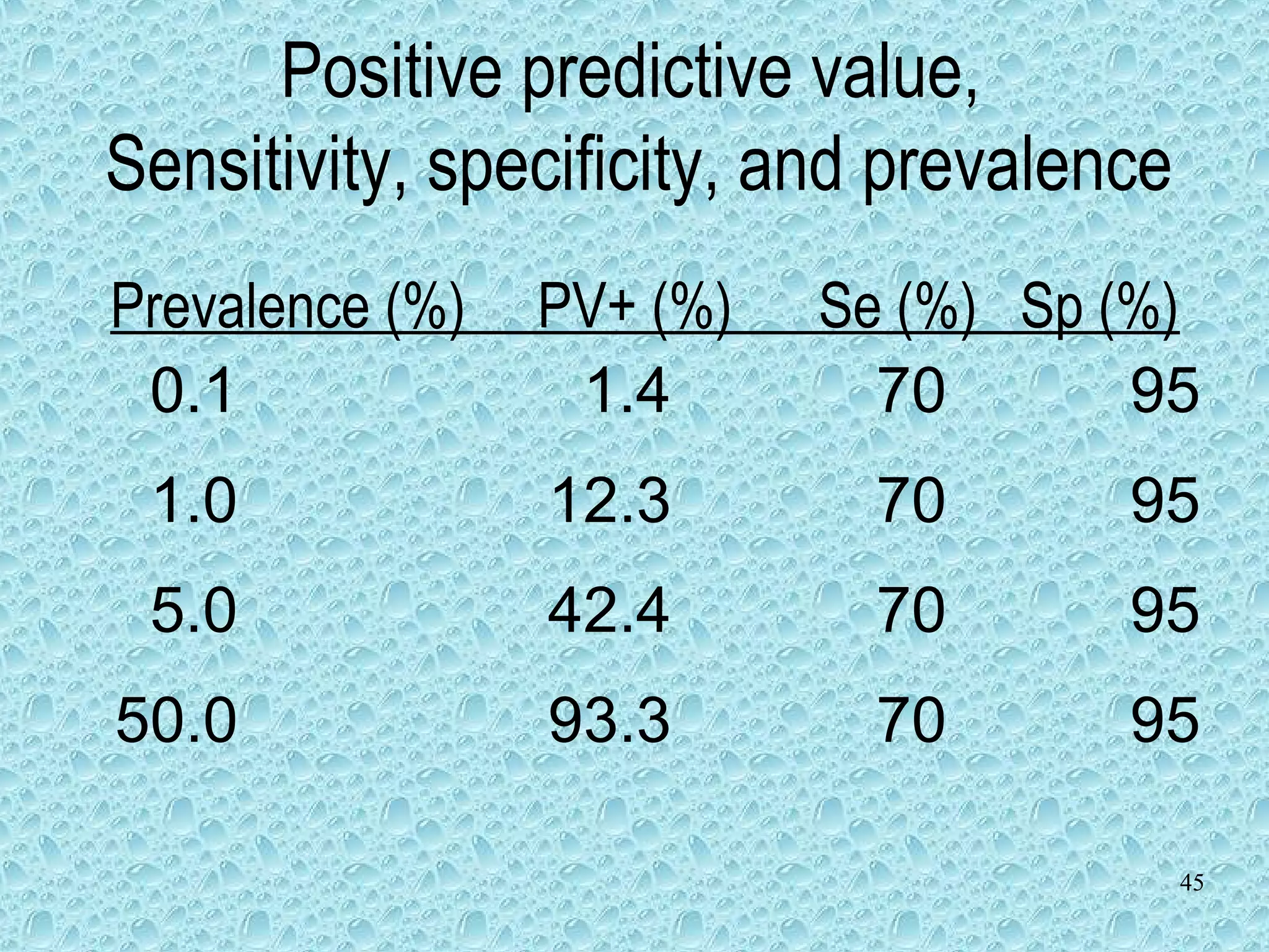
Sensitivity, specificity, and predictive values in the context of diagnostic tests.
Understanding positive and negative predictive values in diagnostic tests.
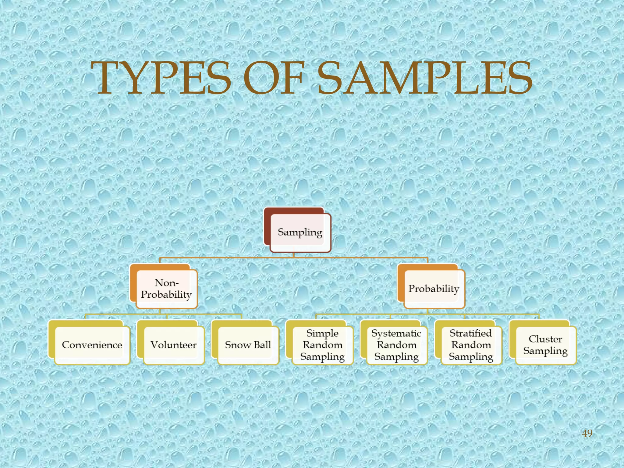
Reasons for sampling, methods, and types of samples.
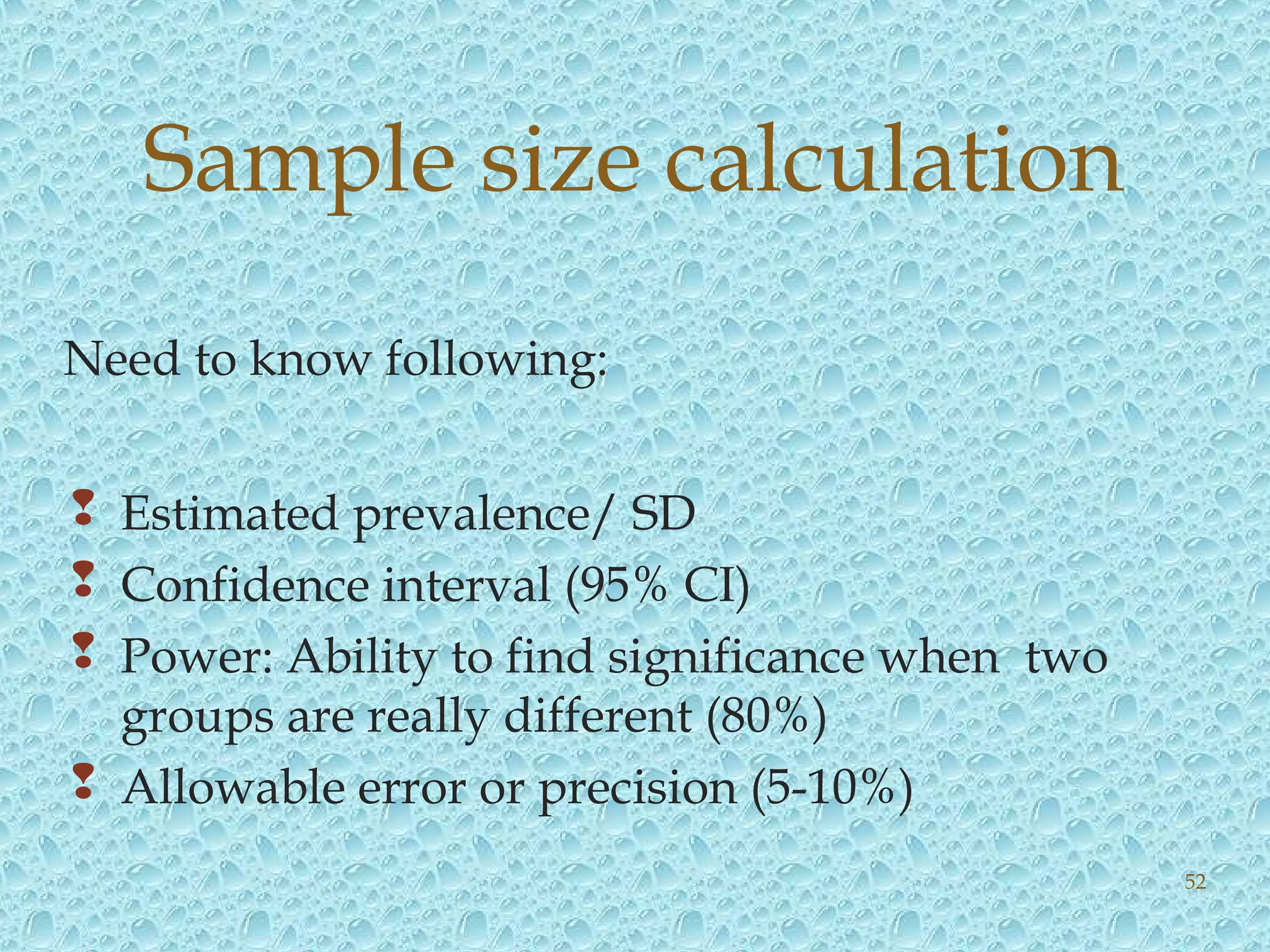
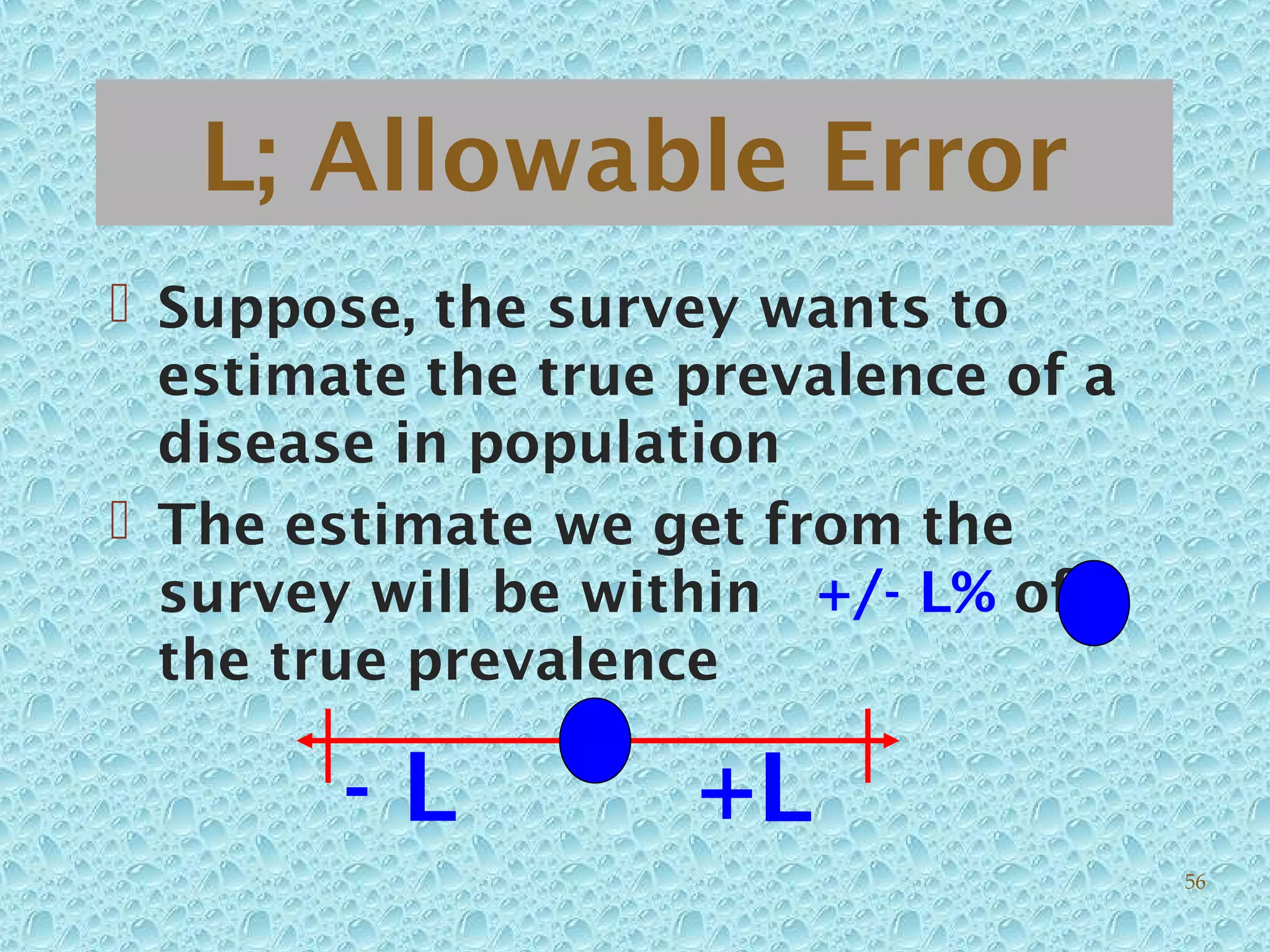
Importance of calculating appropriate sample sizes for reliability in studies.
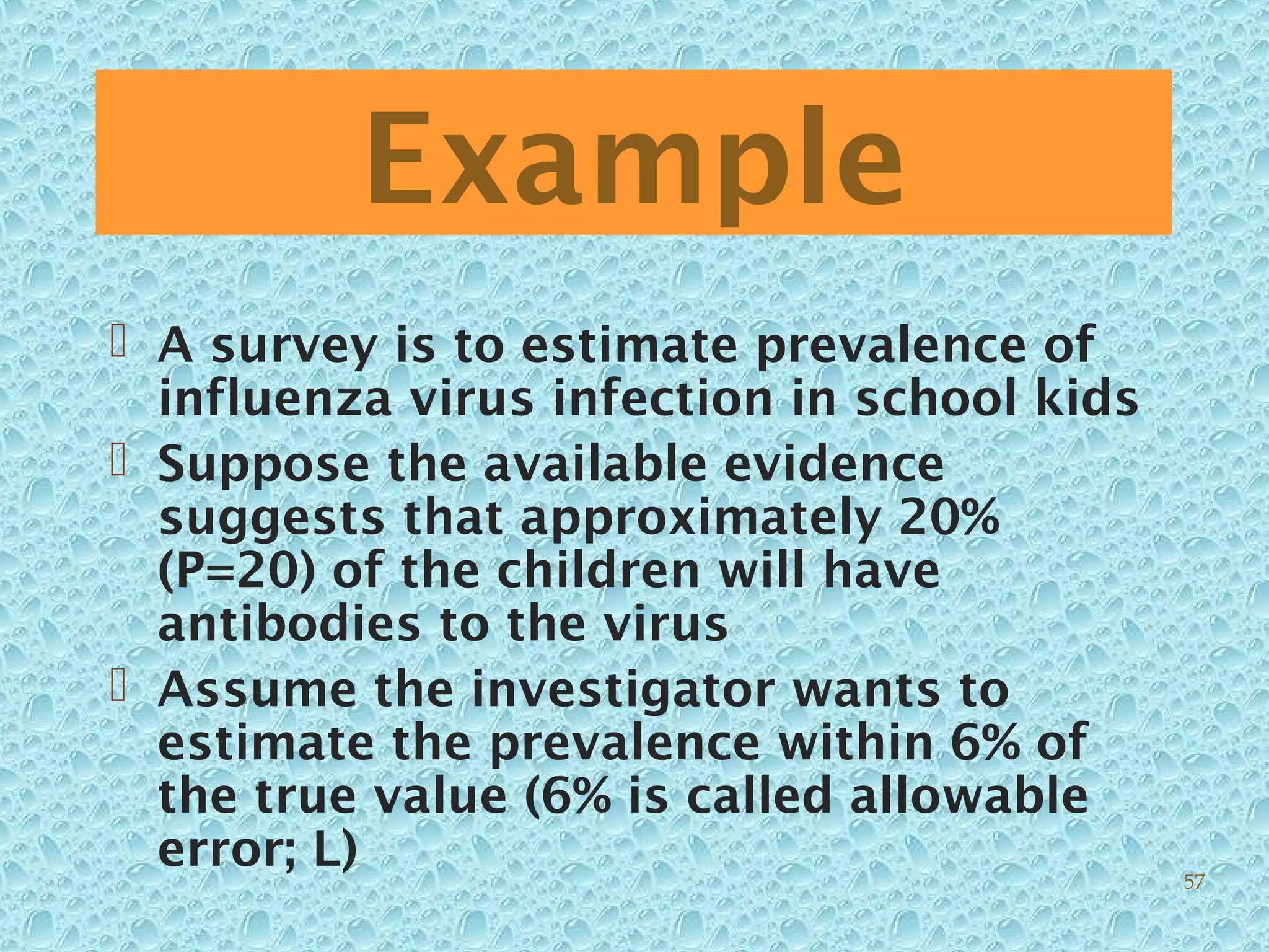
Examples of calculating sample sizes for qualitative and quantitative studies.
Thank you slide to conclude the presentation.