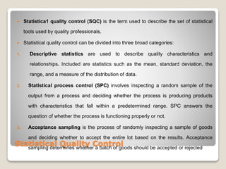
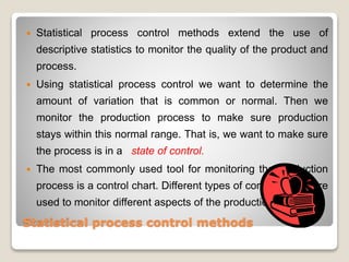
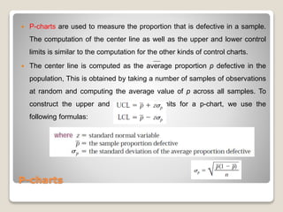
Statistical Process control

Statistical Process
control
Presented by – Prashant Tomar
M.pharmcy QAT
SGRRITS
Presented to – Dr. Praveen k. Chaudhary
H.O.D QAT
Division of Pharmaceutical Sciences,
SGRRITS

Statistical Quality Control
 Statistica1 quality control (SQC) is the term used to describe the set of statistical
tools used by quality professionals.
 Statistical quality control can be divided into three broad categories:
1. Descriptive statistics are used to describe quality characteristics and
relationships. Included are statistics such as the mean, standard deviation, the
range, and a measure of the distribution of data.
2. Statistical process control (SPC) involves inspecting a random sample of the
output from a process and deciding whether the process is producing products
with characteristics that fall within a predetermined range. SPC answers the
question of whether the process is functioning properly or not.
3. Acceptance sampling is the process of randomly inspecting a sample of goods
and deciding whether to accept the entire lot based on the results. Acceptance
sampling determines whether a batch of goods should be accepted or rejected

Statistical process control methods
 Statistical process control methods extend the use of
descriptive statistics to monitor the quality of the product and
process.
 Using statistical process control we want to determine the
amount of variation that is common or normal. Then we
monitor the production process to make sure production
stays within this normal range. That is, we want to make sure
the process is in a state of control.
 The most commonly used tool for monitoring the production
process is a control chart. Different types of control charts are
used to monitor different aspects of the production process.

Developing Control Charts
 A control chart (also called process chart or quality
control chart) is a graph that shows whether a sample of
data falls within the common or normal range of
variation.
 A control chart has upper and lower control limits that
separate common from assignable causes of variation.
The common range of variation is defined by the use of
control chart limits. We say that a process is out of
control when a plot of data reveals that one or more
samples fall outside the control limits.

Developing Control Charts
 The x axis represents samples (#1, #2, #3, etc.) taken from the process
over time. The y axis represents the quality characteristic that is being
monitored (ounces of liquid). The center line (CL) of the control chart is
the mean, or average, of the quality characteristic that is being
measured.
 The upper control limit (UCL) is the maximum acceptable variation from
the mean for a process that is in a state of control. Similarly, the lower
control limit (LCL) is the minimum acceptable variation from the mean
for a process that is in a state of control.
 The upper and lower control limits on a control chart are usually set at
3 standard deviations from the mean. If we assume that the data
exhibit a normal distribution, these control limits will capture 99.74
percent of the normal variation. Control limits can be set at 2 standard
deviations from the mean. In that case, control limits would capture
95.44 percent of the values.

Types of Control Charts
 Control charts are one of the most commonly used tools in statistical
process control. They can be used to measure any characteristic of a
product, such as the weight of a cereal box, the number of chocolates
in a box, or the volume of bottled water.
 The different characteristics that can be measured by control charts
can be divided into two groups: variables and attributes.
 A control chart for variables is used to monitor characteristics that can
be measured and have a continuum of values, such as height, weight,
or volume.
 A control chart for attributes, on the other hand, is used to monitor
characteristics that have discrete values and can be counted. Often
they can be evaluated with a simple yes or no decision. Examples
include color, taste, or smell.

Control Charts For Variables
 Control charts for variables monitor characteristics that can
be measured and have a continuous scale, such as height,
weight, volume, or width. When an item is inspected, the
variable being monitored is measured and recorded.
 Two of the most commonly used control charts for variables
monitor both the central tendency of the data (the mean) and
the variability of the data (either the standard deviation or the
range). Each chart monitors a different type of information.
 When observed values go outside the control limits, the
process is assumed not to be in control. Production is
stopped, and employees attempt to identify the cause of the
problem and correct it.

Mean (x-Bar) Charts
 A mean control chart is often referred to as an x-bar chart. It is
used to monitor changes in the mean of a process.
 To construct a mean chart we first need to construct the center line
of the chart. To do this we take multiple samples and compute their
means. Usually these samples are small, with about four or five
observations. Each sample has its own mean. The center line of the
chart is then computed as the mean of all sample means :
 To construct the upper and lower control limits of the chart, we use
the following formulas:

Mean (x-Bar) Charts
Cont....
• Another way to construct the control limits is to use the sample range as an estimate
of the variability of the process. Range is simply the difference between the largest
and smallest values in the sample. The spread of the range tell about the variability
of the data. In this case control limits would be constructed as follows:

Range (R) Charts
 Range (R) charts are another type of control chart for
variables. Whereas x-bar charts measure shift in the
central tendency of the process, range charts monitor
the dispersion or variability of the process. The method
for developing and using R-charts is the same as that
for x-bar charts. The center line of the control chart is
the average range, and the upper and lower control
limits are computed as follows:

Using Mean and Range Charts Together
 The mean or x-bar chart measures the central tendency of the
process, whereas the range chart measures the dispersion or
variance of the process. Since both variables are important, it
makes sense to monitor a process using both mean and range
charts.

Control charts for attributes
 Control charts for attributes are used to measure quality characteristics that are
counted rather than measured. Attributes are discrete in nature and entail simple
yes-or-no decisions. For example, this could be the number of nonfunctioning light
bulbs, the proportion of broken eggs in a carton, the number of rotten apples, the
number of scratches on a tile, or the number of complaints issued.
 Two of the most common types of control charts for attributes are p-charts and c-
charts.
 P-charts are used to measure the proportion of items in a sample that are defective.
Examples are the proportion of broken cookies in a batch and the proportion of cars
produced with a misaligned fender. P-charts are appropriate when both the number
of defectives measured and the size of the total sample can be counted. A proportion
can then be computed and used as the statistic of measurement.
 C-charts count the actual number of defects. For example, we can count the number
of complaints from customers in a month, the number of bacteria on a Petri dish.
However, we cannot compute the proportion of complaints from customers, the
proportion of bacteria on a Petri dish.

P-charts
 P-charts are used to measure the proportion that is defective in a sample.
The computation of the center line as well as the upper and lower control
limits is similar to the computation for the other kinds of control charts.
 The center line is computed as the average proportion p defective in the
population, This is obtained by taking a number of samples of observations
at random and computing the average value of p across all samples. To
construct the upper and lower control limits for a p-chart, we use the
following formulas:

C-charts
 C-charts are used to monitor the number
of defects per unit. Example the number
of returned meals in a restaurant.
 The average number of defects c , is the
center line of the control chart. The upper
and lower control limits are computed as
follows:

Summary of SPC
 We have discussed several types of statistical quality control (SQC) techniques.
 One category of SQC techniques consists of descriptive statistics tools such as the
mean, range, and standard deviation. These tools are used to describe quality
characteristics and relationships.
 Another category of SQC techniques consists of statistical process control (SPC)
methods that are used to monitor changes in the production process. To understand
SPC methods we must understand the differences between common and assignable
causes of variation. Common causes of variation are based on random causes that
cannot be identified.
 A certain amount of common or normal variation occurs in every process due to
differences in materials, workers, machines, and other factors.
 Assignable causes of variation, on the other hand, are variations that can be
identified and eliminated. An important part of statistical process control (SPC) is
monitoring the production process to make sure that the only variations in the
process are those due to common or normal causes.
 Under these conditions we say that a production process is in a state of control.
 We also understood the different types of quality control charts that are used to
monitor the production process: x-bar charts, R-range charts, p-charts, and c-charts.

Process capability
 Process capability is the ability of a production
process to meet or exceed preset specifications.
 Product specifications preset ranges of
acceptable quality characteristics.
 Process capability involves evaluating process
variability relative to preset product
specifications in order to determine whether the
process is capable of producing an acceptable
product.

Measuring Process Capability
 Simply setting up control charts to monitor whether a process is in control does
not guarantee process capability. To produce an acceptable product, the
process must be capable and in control before production begins.
 Process capability is measured by the process capability index, Cp, which is
computed as the ratio of the specification width to the width of the process
variability:
 where the specification width is the difference between the upper specification
limit (USL) and the lower specification limit (LSL) of the process. The process
width is computed as 6 standard deviations of the process being monitored.

 There are three possible ranges of values for Cp that also
help us interpret its value:
 A value of Cp equal to 1 means that the process variability
just meets specifications. We would then say that the process
is minimally capable.
 A value of Cp below 1 means that the process variability is
outside the range of specification. This means that the
process is not capable of producing within specification and
the process must be improved.
 A value of Cp above 1 means that the process variability is
tighter than specifications and the process exceeds minimal
capability.

 Cp is valuable in measuring process capability. However, it has one
shortcoming: it assumes that process variability is centered on the
specification range. Unfortunately, this is not always the case.
 Figure shows data from the Cocoa Fizz example. In the figure the
specification limits are set between 15.8 and 16.2 ounces, with a
mean of 16.0 ounces. However, the process variation is not
centered; it has a mean of 15.9 ounces. Because of this, a certain
proportion of products will fall outside the specification range.

 Because of this, another measure for process capability is
used more frequently:
 This measure of process capability helps us address a
possible lack of centering of the process over the
specification range. To use this measure, the process
capability of each half of the normal distribution is computed
and the minimum of the two is used.

Six Sigma Quality
 The term Six Sigma was coined by the Motorola
Corporation in the 1980s to describe the high
level of quality the company was striving to
achieve. Sigma stands for the number of
standard deviations of the process.
 3 sigma means that 2600 ppm are defective.
The level of defects associated with Six Sigma
is approximately 3.4 ppm, because 3 sigma
considers 99.74% of normal variation and
0,26% defective which in ppm is around 2600
ppm.
 The level of defects associated with Six Sigma
is approximately 3.4 ppm.

Six Sigma Quality
There are two aspects to implementing the Six Sigma concept. The first is the
use of technical tools to identify and eliminate causes of quality problems.
These technical tools include the statistical quality control tools. They also
include the problem-solving tools such as cause-and-effect diagrams, flow
charts, and Pareto analysis. In Six Sigma programs the use of these technical
tools is integrated throughout the entire organizational system
The second aspect of Six Sigma implementation is people involvement. In Six
Sigma all employees have the training to use technical tools and are
responsible for rooting out quality problems.

References
 Brue, G. Six Sigma for Managers. New York:
McGraw-Hill, 2002.
 Duncan, A. J. Quality Control and Industrial
Statistics. 5th ed.Homewood, Ill.: Irwin, 1986.
 Evans, James R., and William M. Lindsay. The
Management and Control of Quality. 4th ed.
Cincinnati: South-Western, 1999.
 Feigenbaum, A. V. Total Quality Control. New York:
McGraw-Hill, 1991.
 Grant, E. L., and R. S. Leavenworth. Statistical
Quality Control.6th ed. New York:McGraw-Hill, 1998

Statistical Process control

More Related Content

What's hot

Viewers also liked

Similar to Statistical Process control

Recently uploaded

Statistical Process control