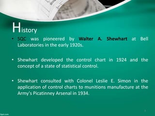
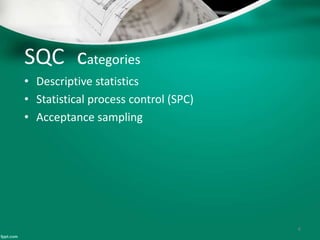
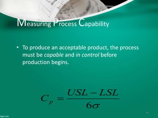
Statistical quality control (SQC) refers to the statistical tools used by quality professionals. SQC was pioneered in the 1920s by Walter Shewhart who developed control charts. Shewhart consulted on applying control charts during WWII. W. Edwards Deming helped introduce SQC methods to American and Japanese industry. SQC includes descriptive statistics, statistical process control (SPC), and acceptance sampling. Descriptive statistics describe quality characteristics while SPC uses control charts to monitor processes and determine if they are in a state of statistical control. Acceptance sampling involves inspecting samples to determine if full lots meet standards.

1. Statistical Quality Control
1

2. What is SQC ?
• Statistical quality control (SQC) is the term
used to describe the set of statistical tools
used by quality professionals.
2

3. History
• SQC was pioneered by Walter A. Shewhart at Bell
Laboratories in the early 1920s.
• Shewhart developed the control chart in 1924 and the
concept of a state of statistical control.
• Shewhart consulted with Colonel Leslie E. Simon in the
application of control charts to munitions manufacture at the
Army's Picatinney Arsenal in 1934.
3

4. History
• W. Edwards Deming invited Shewhart to speak at
the Graduate School of the U.S. Department of
Agriculture, and served as the editor of Shewhart's
book Statistical Method from the Viewpoint of Quality
Control (1939) which was the result of that lecture.
• Deming was an important architect of the quality
control short courses that trained American
industry in the new techniques during WWII.
4

5. • Deming traveled to Japan during the Allied
Occupation and met with the Union of Japanese
Scientists and Engineers(JUSE)in an effort to
introduce SQC methods to Japanese industry
5

6. SQC categories
6
• Descriptive statistics
• Statistical process control (SPC)
• Acceptance sampling

7. Descriptive Statistics
• Descriptive statistics are used to describe quality
characteristics and relationships.
7

8. Descriptive Statistics
– The Mean- measure of central tendency
– The Range- difference between largest/smallest
observations in a set of data
– Standard Deviation measures the amount of data
dispersion around mean
8

9. The Mean
• To compute the mean we simply sum all the observations and divide by the total
no. of observations.
9

10. The Range
• Range, which is the difference between the largest
and smallest observations.
10

11. Standard Deviation
• Standard deviation is a measure of dispersion of
a curve.
• It measures the extent to which these values are
scattered around the central mean.
11

12. • Extend the use of descriptive statistics to monitor
the quality of the product and process
• Statistical process control help to determine the
amount of variation
• To make sure the process is in a state of control
12
Statistical process control
12

13. Variation in Quality
• No two items are exactly alike.
• Some sort of variations in the two items is bound to be
there. In fact it is an integral part of any manufacturing
process.
• This difference in characteristics known as variation.
• This variation may be due to substandard quality of raw
material, carelessness on the part of operator, fault in
machinery system etc..
13

14. Types Of Variations
14
• Variation due to “CHANCE CAUSES”
• Variation due to “ASSIGNABLE CAUSES”

15. Variation due to chance causes/common causes
• Variation occurred due to chance.
• This variation is NOT due to defect in machine,
Raw material or any other factors.
• Behave in “random manner”.
• Negligible but Inevitable
• The process is said to be under the state of
statistical control.
15
15

16. Variation due to assignable causes
Non – random causes like:
– Difference in quality of raw material
– Difference in machines
– Difference in operators
– Difference of time
16
16

17. 17

18. Specification and control limits
• No item in the world can be a true copy of another item.
• It is not expressed in absolute values but in terms of a
range.
• For Eg:
The diameter of a pen is expected by its manufacturer
not as 7mm but as 7mm ± 0.05.
Thus, the diameter of a pen produced by the
manufacturer can vary from 6.95 mm to 7.05 mm.
18

19. Setting Control Limits
19

20. HOW CONTROL LIMITS ARE USEFUL…..?
20

21. SPC Methods-Control Charts
• Control Charts show sample data plotted on a graph
with CL, UCL, and LCL
• Control chart for variables are used to monitor
characteristics that can be measured, e.g. length,
weight, diameter, time
• Control charts for attributes are used to monitor
characteristics that have discrete values and can be
counted, e.g. % defective, number of flaws in a shirt,
number of broken eggs in a box
21

22. Control Charts for Variables
• x-bar charts
It is used to monitor the changes in the mean of
a process (central tendencies).
• R-bar charts
It is used to monitor the dispersion or variability
of the process
22

23. Constructing a X-bar chart
• A factory produces 50 cylinders per hour. Samples of 10 cylinders
are taken at random from the production at every hour and the
diameters of cylinders are measured. Draw X-bar and R charts and
decide whether the process is under control or not.
23

24. Sample no. x1 x2 x3 x4
1 230 238 242 250
2 220 230 218 242
3 222 232 236 240
4 250 240 230 225
5 228 242 235 225
6 248 222 220 230
7 232 232 242 242
8 236 234 235 237
9 231 248 251 271
10 220 222 224 231
24

25. Sample
no.
x1 x2 x3 x4 Sigma
Xi
Mean
X-bar
Range
R
1 230 238 242 250 960 240.00 20
2 220 230 218 242 910 227.50 24
3 222 232 236 240 930 232.50 18
4 250 240 230 225 945 236.25 25
5 228 242 235 225 930 232.50 17
6 248 222 220 230 920 230.00 28
7 232 232 242 242 948 237.00 10
8 236 234 235 237 942 235.50 3
9 231 248 251 271 1001 250.25 40
10 220 222 224 231 897 224.25 11
Total 2345.75 196
25

26. Calculation of x-bar and R-bar
• Now,
26
75.234
10
75.2345
m

x
x
6.19
10
196


m
R
R

27. 27
Factor for x-Chart
A2 D3 D4
2 1.88 0.00 3.27
3 1.02 0.00 2.57
4 0.73 0.00 2.28
5 0.58 0.00 2.11
6 0.48 0.00 2.00
7 0.42 0.08 1.92
8 0.37 0.14 1.86
9 0.34 0.18 1.82
10 0.31 0.22 1.78
11 0.29 0.26 1.74
12 0.27 0.28 1.72
13 0.25 0.31 1.69
14 0.24 0.33 1.67
15 0.22 0.35 1.65
Factors for R-Chart
Sample Size
(n)
Factors for calculating control limits

28. Control limits of X-BarChart
• Central line C.L =
• U.C.L =
=234.75 + (0.73) (19.6)
=249.06
• L.C.L=
=234.75- (0.73) (19.6)
=220.72
28
RAx *2
RAx *2
75.234x
For n = 4 A2=0.73

29. X-BarChart
29

30. Control limits of R-BarChart
• Central Line =
• U.C.L =
=45.50
• L.C.L =
=0
30
6.19R
)96.19(*)28.2(4 RD
)96.19(*)0(3 RD
For n = 4, D4=2.28, D3=0

31. R-BarChart
31

32. Control Charts for Attributes
• Attributes are discrete events; yes/no, pass/fail
Use P-Charts for quality characteristics that are discrete and
involve yes/no or good/bad decisions
• Number of leaking caulking tubes in a box of 48
• Number of broken eggs in a carton
Use C-Chartsfor discrete defects when there can be more
than one defect per unit
• Number of flaws or stains in a carpet sample cut from a
production run
• Number of complaints per customer at a hotel
32

33. P-Chart Example
• A Production manager of a BKT tire company has inspected the
number of defective tires in five random samples with 20 tires in
each sample. The table below shows the number of defective tires
in each sample of 20 tires. Calculate the control limits.
33

34. 34

35. 35

36. P- Control Chart
36

37. C - Chart Example
• The number of weekly customer complaints are monitored in a
large hotel using a c-chart. Develop three sigma control limits
using the data table below.
37

38. 38

39. 39

40. C - Control Chart
40

41. Process Capability
• Evaluating the ability of a production process to meet or exceed
preset specifications. This is called process capability.
• Product specifications, often called tolerances, are preset ranges of
acceptable quality characteristics, such as product dimensions.
41

42. Two parts of process capability
1) Measure the variability of the output of a process,
and
2) Compare that variability with a proposed
specification or product tolerance.
42

43. Measuring Process Capability
• To produce an acceptable product, the process
must be capable and in control before
production begins.
43
6
LSLUSL
Cp



44. Example
• Let’s say that the specification for the
acceptable volume of liquid is preset at 16
ounces ±.2 ounces, which is 15.8 and 16.2
ounces.
44

45. Figure (a)
• The process produces 99.74 percent (three sigma) of the product
with volumes between 15.8 and 16.2 ounces.
45
1pC

46. Figure (b)
• The process produces 99.74 percent (three
sigma) of the product with volumes between
15.7 and 16.3 ounces.
46
1pC

47. Figure (c)
• the production process produces 99.74 percent (three sigma) of the
product with volumes between 15.9 and 16.1 ounces.
47
1pC

48. Process capability ratio (off centering process)
• There is a possibility that the process mean may
shift over a period of time, in either direction,
i.e., towards the USL or the LSL. This may result
in more defective items then the expected. This
shift of the process mean is called the off-
centering of the process.
48





 





3
,
3
min
LSLUSL
C kp

49. Example
• Process mean:
• Process standard deviation:
• LSL = 15.8
• USL = 16.2
49
9.15
067.0
1
)067.0(6
4.0
pC

50. 




 





3
,
3
min
LSLUSL
C kp
50
33.0
33.0,00.1min
)1(.3
8.159.15
,
)1(.3
9.152.16
min











 

pk
pk
kp
C
C
C

51. Thank You…
51