Spatial interpolation comparison

Spatial Interpolation Comparison
Evaluation of spatial prediction methods
Tomislav Hengl
ISRIC — World Soil Information, Wageningen University
Geostatistics course, 25–29 October 2010, Wageningen

Based on
Hengl, T., MacMillan, R.A., 2011? Mapping eﬃciency and
information content. submitted to International Journal of
Applied Earth Observation and Geoinformation, special issue
Spatial Statistics Conference.

Topic
Geostatistics = a toolbox to generate maps from point data
i.e.to interpolate;

Topic
i.e.to interpolate;
There are many possibilities;

Topic
i.e.to interpolate;
An inexperienced user will often be challenged by the amount
of techniques to run spatial interpolation;

Topic
i.e.to interpolate;
An inexperienced user will often be challenged by the amount
of techniques to run spatial interpolation;
. . .which method should we use?

Have you heard of SIC?

The spatial prediction game
Participants were invited to estimate values located at 1000
locations (right, crosses), using 200 observations (left, circles).

Lessons learned (from SIC)

Li and Heap (2008)

How many techniques are there?
Li and Heap (2008) list over 40 unique techniques.
1. Are all these equally valid?
2. How to objectively compare various methods (which criteria
to use)?
3. Which method to pick for your own case study?

There are not as many
There are roughly ﬁve main clusters of techniques:
1. splines (deterministic);

2. kriging-based (plain geostatistics);

3. regression-based;

4. bayesian methods;

4. bayesian methods;
5. expert systems / machine learning;

The 5 criteria
1. the overall mapping accuracy, e.g.standardized RMSE at
control points — the amount of variation explained by the
predictor expressed in %;

The 5 criteria
2. the bias, e.g.mean error — the accuracy of estimating the
central population parameters;

The 5 criteria
3. the model robustness, also known as model sensitivity — in
how many situations would the algorithm completely fail /
how much artifacts does it produces?;

The 5 criteria
4. the model reliability — how good is the model in estimating
the prediction error (how accurate is the prediction variance
considering the true mapping accuracy)?;

The 5 criteria
4. the model reliability — how good is the model in estimating
the prediction error (how accurate is the prediction variance
considering the true mapping accuracy)?;
5. the computational burden — the time needed to complete
predictions;

Can we simplify this?
1. In theory, we could derive a single composite measure that
would then allow you to select ‘the optimal’ predictor for any
given data set (but this is not trivial!)
2. But how to assign weights to diﬀerent criteria?
3. In many cases we simply ﬁnish using some na¨ıve predictor —
that is predictor that we know has a statistically more optimal
alternative, but this alternative is not feasible.

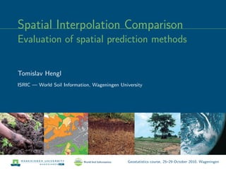
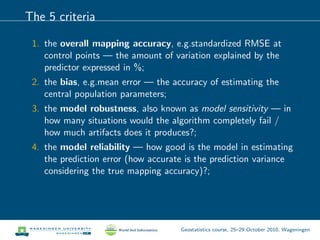
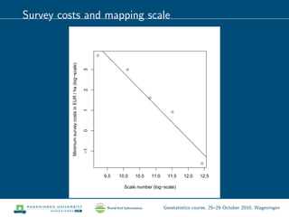
Automated mapping
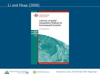
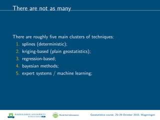
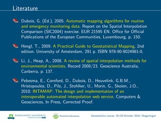
In the intamap package1 decides which method to pick for you:
> meuse$value <- log(meuse$zinc)
> output <- interpolate(data=meuse, newdata=meuse.grid)
R 2009-11-11 17:09:14 interpolating 155 observations,
3103 prediction locations
[Time models loaded...]
[1] "estimated time for copula 133.479866956255"
Checking object ... OK
1
http://cran.r-project.org/web/packages/intamap/

Hypothesis
We need a single criteria to compare various prediction methods.

Mapping accuracy and survey costs
The cost of a soil survey is also a function of mapping scale,
roughly:
log(X) = b0 + b1 · log(SN) (1)
We can ﬁt a linear model to the empirical table data from
e.g.Legros (2006; p.75), and hence we get:
X = exp (19.0825 − 1.6232 · log(SN)) (2)
where X is the minimum cost/ha in Euros (based on estimates in
2002). To map 1 ha of soil at 1:100,000 scale, for example, one
needs (at least) 1.5 Euros.

Survey costs and mapping scale
q
q
q
q
q
9.5 10.0 10.5 11.0 11.5 12.0 12.5
−10123
Scale number (log−scale)
MinimumsurveycostsinEUR/ha(log−scale)

Survey costs and mapping scale
Total costs of a soil survey can be estimated by using the size of
area and number of samples.
The eﬀective scale number (SN) is:
SN = 4 ·
A
N
· 102
. . . SN =
A
N
· 102
(3)
where A is the surface of the study area in m2 and N is the total
number of observations.

Converges to:
X = exp 19.0825 − 1.6232 · log 0.0791 ·
A
N
· 102
(4)

Output map, from info perspective
The resulting (predictions) map is a sum of two signals:
Z∗
(s) = Z(s) + ε(s) (5)
where Z(s) is the true variation, and ε(s) is the error component.
The error component consists, in fact, of two parts: (1) the
unexplained part of soil variation, and (2) the noise (measurement
error). The unexplained part of soil variation is the variation we
somehow failed to explain because we are not using all relevant
covariates and/or due to the limited sampling intensity.

Prediction accuracy
In order to see how much of the global variation budget has been
explained by the model we can use:
RMSEr (%) =
RMSE
sz
· 100 (6)
where sz is the sampled variation of the target variable.
RMSEr (%) is a global estimate of the map accuracy, valid only
under the assumption that the validation points are spatially
independent from the calibration points, representative and large
enough ( 100).

Kriging eﬃciency

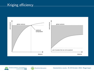
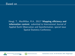
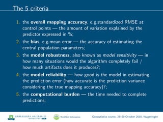
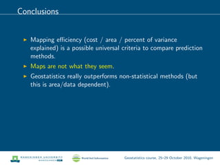
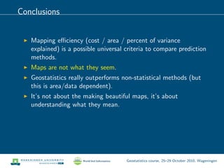
Mapping efficiency
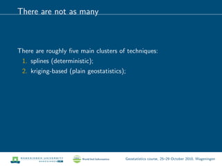
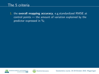
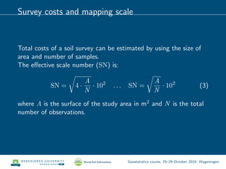
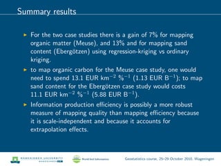
We propose two new measures of mapping success: (1) Mapping
efficiency, defined as the amount of money needed to map an area
of standard size and explain each one percent of variation in the
target variable:
θ =
X
A · RMSEr
[EUR · km−2
· %−1
] (7)
where X is the total costs of a survey, A is the size of area in
km−2, and RMSEr is the amount of variation explained by the
spatial prediction model.

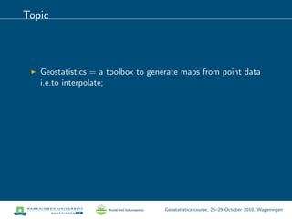
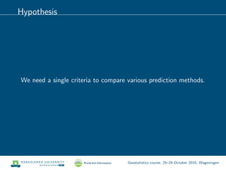
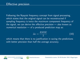
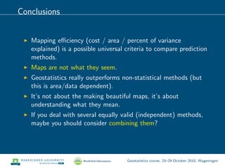
Information production efficiency
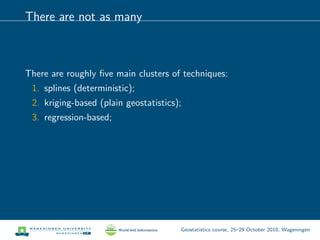
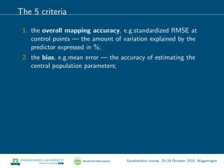
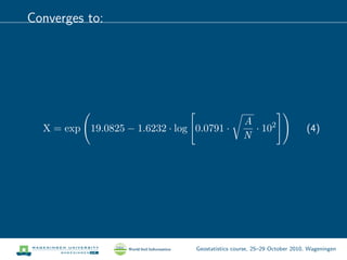
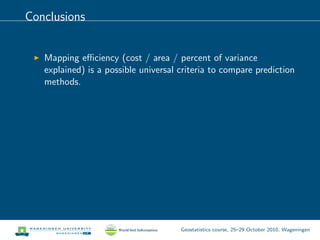
(2) Equivalent measure of mapping efficiency is the information
production efficiency:
Υ =
X
gzip
[EUR · B−1
] (8)
where gzip is the size of data (in Bytes) left after compression and
after reformatting the values to match the effective precision
(based on Eq.10). This can be estimated as:
gzip = fc · (fE · M ) · cZ [B] (9)
where fc is the loss-less data compression factor that depends on
the compression algorithm, fE is the extrapolation adjustment
factor, cZ is the variable coding size, and M is the total number of
pixels.

Effective precision
Following the Nyquist frequency concept from signal processing,
which states that the original signal can be reconstructed if
sampling frequency is twice the maximum component frequency of
the signal, we can derive the effective precision — also known as
numerical resolution — of a produced prediction map as:
∆z =
RMSE
2
(10)
which means that there is no justification in saving the predictions
with better precision than half the average accuracy.

Nyquist frequency concept
q
q
qq
q
qq q
q
q
q
q q
qqq
q
q qq
q
qq q
q
q
q
q
q
qq
q
q
q q
q
q
q q qqq q q
q
q
qq
Figure: The Nyquist rate is the optimal rate that can be used to
compress a signal (it equals twice the maximum component frequency of
the signal) to allow perfect reconstruction of the signal from the samples.

Rounding numbers
Original data
2.25 4.08 6.25 4.23 2.56 1.21 0.98 0.98 0.85 0.4
4.24 4.69 7.17 4.37 2.08 1.4 1.44 0.96 0.89 0.31
3.62 5.39 5.27 3.11 2.04 1.57 1.67 1.43 0.61 0.28
2.72 8.75 7.77 4.63 2.88 2.34 2.93 1.49 0.57 0.25
2.83 10.55 14.45 5.79 3.13 2.95 2.85 0.89 0.34 0.22
2.87 5.45 10.34 5.01 2.42 1.88 1.5 0.61 0.3 0.23
1.19 2.69 3.76 3.63 1.86 0.97 1.24 0.64 0.37 0.26
0.86 1.22 1.39 2.71 2.17 1.61 2.37 1.56 0.66 0.47
0.67 1 1.23 1.53 2.04 3.12 5.74 3.71 1.53 0.92
1.18 1.48 1.35 2.13 2.11 3.64 7.56 6.92 2.97 1.96
Coded data
2 4 6 4 3 1 1 0
5 7 4 2 1 1 0
4 5 5 2 2 2 1 1
3 9 8 5 3 2 3 1 1
3 11 14 6 3 3 3
3 5 10 5 2 2 1
1 3 4 4 2 1 0
1 3 2 2 2
1 1 2 2 3 6 4 2 1
1 1 2 2 4 8 7 3 2

Exercise
To follow this exercise, obtain the DSM_examples.R script.
Download it to your machine and then run step-by-step.

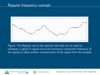
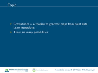
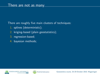
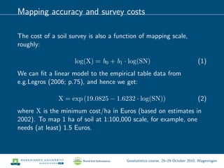
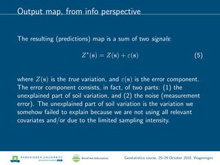
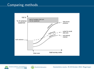
Meuse data
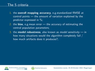
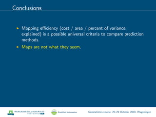
> data(meuse)
> coordinates(meuse) <- ~x+y
> proj4string(meuse) <- CRS("+init=epsg:28992")
> sel <- !is.na(meuse$om)
> bubble(meuse[sel,], "om")
om
qqqq
qq
qq
q qq
q
qq
qq
q
q
q
qqqq
q
qqq
q
q
q
q
q
q
q
qq
q
qq
q
q
q
q
q
q
q
q
qq
qqqqq
q
q
q
q
q
q
q
q
qq
q
q
q
q
qq
qq
qq
q
q
q
qq
q
q
q
q
q
q
q
q
q qq
q
qq
q
qq
q
q q
q
q
q
q
q
q
q
q
qq
q
q
qq
q
q
q
q
q
qq
q
q
q
q
q
q
q
q
q
q
q
q
q
q
q
qq
q
q q
q
qq
qq
q q
q
q
qq q
q
q
q
q
q
q
1
5.3
6.9
9
17

Meuse
+
+ +
+
+
+
++
+
+
+
+
+
+
+
+
+
+
+
+ +++
+
+++
+
+
+
+
++
+
++
+
++
+
+
++
+
+
+
+
+
+
++
+
+++
+
+
+
+
+
+
+
+
+
+
+
+
+
+
+
++
+ +
++
+
+
+
+
+
+
+
+
+
+
+
+
+
+ ++
+
+
+
+
++
+
+
+
+
+
+
+
+
+
+
+
++
+
+
++
+
+
+
+
+
++
+
+
+
+
+
+
+
+
+
+
+
+
+
+
+
++
+
+ +
+
+
+
++
+
+
+
+
++
+
+
om.ok
+
+ +
+
+
+
++
+
+
+
+
+
+
+
+
+
+
+
+ +++
+
+++
+
+
+
+
++
+
++
+
++
+
+
++
+
+
+
+
+
+
++
+
+++
+
+
+
+
+
+
+
+
+
+
+
+
+
+
+
++
+ +
++
+
+
+
+
+
+
+
+
+
+
+
+
+
+ ++
+
+
+
+
++
+
+
+
+
+
+
+
+
+
+
+
++
+
+
++
+
+
+
+
+
++
+
+
+
+
+
+
+
+
+
+
+
+
+
+
+
++
+
+ +
+
+
+
++
+
+
+
+
++
+
+
om.rk
0
2
4
6
8
10
12
14

Eberg¨otzen (subset)
+
+
+
+
+
+
+
+
+
+
+ +
+
+
+
+
+
+
+
+
+
+
+
+ +
+ +
+
+
+
+
+
++
+
+
+
+
+
+
+
+
+
+
+
+
+
+
+
+
+
+
+
+
+
+
++
+
+
+
+++
+
+
+
+
++
+
+
+
+
+
+
+
+
+
+
+
+
+
+
+
+
+
+
+
+
+
+
+
+
+
+
+
+
+
+
+
+
+
+
+
+
+
+
+
+
+
+
+
+
+
+
+
++
+
+
+
+
+
+
+
+
+
+
+
+
+
+
+
+
+
+
++
+
+
+
+
+
+
+
+
+
+
+
+
+
++
+
+++
+
+
+
+
+
+
+
+
+
+
+
+
+
+
+
+ +
+
+
+
+
+
+
+
+
+
+
+
+
+
+
+
+
+
+
+
+
+
+
+
+
+
+
+
+
+
+
+
+
+
+
+
+
+
+
+
+
+
+
+
+
+
+
+
+
+
+
+
+
+
+
+
+
+
+
+
+
+
+
+
+
+
+
+
+
+
+
+
+
+
+
+
+
+
++
+
+
+
+
+
+
+
+
+
+
+
+
+
+
+
+
+
++
+
++
+
+
+
+
+
+
++
+
+
+
+
+
+
+
+
+
+
+
+
+
+
+
+
+
SAND.ok.1
+
+
+
+
+
+
+
+
+
+
+ +
+
+
+
+
+
+
+
+
+
+
+
+ +
+ +
+
+
+
+
+
++
+
+
+
+
+
+
+
+
+
+
+
+
+
+
+
+
+
+
+
+
+
+
++
+
+
+
+++
+
+
+
+
++
+
+
+
+
+
+
+
+
+
+
+
+
+
+
+
+
+
+
+
+
+
+
+
+
+
+
+
+
+
+
+
+
+
+
+
+
+
+
+
+
+
+
+
+
+
+
+
++
+
+
+
+
+
+
+
+
+
+
+
+
+
+
+
+
+
+
++
+
+
+
+
+
+
+
+
+
+
+
+
+
++
+
+++
+
+
+
+
+
+
+
+
+
+
+
+
+
+
+
+ +
+
+
+
+
+
+
+
+
+
+
+
+
+
+
+
+
+
+
+
+
+
+
+
+
+
+
+
+
+
+
+
+
+
+
+
+
+
+
+
+
+
+
+
+
+
+
+
+
+
+
+
+
+
+
+
+
+
+
+
+
+
+
+
+
+
+
+
+
+
+
+
+
+
+
+
+
+
++
+
+
+
+
+
+
+
+
+
+
+
+
+
+
+
+
+
++
+
++
+
+
+
+
+
+
++
+
+
+
+
+
+
+
+
+
+
+
+
+
+
+
+
+
SAND.rk.1
0
10
20
30
40
50
60
70
80
90

Eberg¨otzen (subset)
+
+
+
+
+
+
+
+
+
+
+
+
+
+
+
+
++
+
+
+
+
+
+
+
+
+
+
+
+
+
+
+
+
+
+
+
+
+
+
+
+
+
+
+
+
+
+
++
+
+
+
++
+
+
+
+
+
+
+
+
+
+
+
+
++
+++
+
+
+
+
+
+
+
+
+
++ +
+
+
+
+
+
+
+
+
+
+
+
+
+
+
+
+
+
+
+
+
+
+
+
+
+
+
+
+
+
+
+
+
+
+++
+
+
+
+
+
+
++
+
+
+
+
+
+
+
+
+
+
+
+
+
+
+
+
+
+
+
+
+
+
+
+
+
+
+
+
+
+
+
+
+
+
+
+
+
+
+
+
+
+
+
++
+
+
+
+
+
+
+
+
+
+
+
+
+
+
+
+
+
+
+
+
+
+
+
+
+
+
+
+
+
+
+
+
+
+
+
+
+
+
+
+
+
+
+
+
+
+
+
+
+
++
+
+
++
+
+
+
+
+
+
+
+
+
+
+
+
+
+
+
+
+
+
+
+
+
+
+
+
+
+
+
+
+
+
+
+
+
+
+
+
+
+
+
+
+
+
+
++
++
+
+
+
++
+
+
+
+
+
+
+
+
+
+
+
+
+
+
+
+
+
+
+
+
+
++
+
+
+
+
++
+
+
+
+
+
+
+
+
+
+
+
+
+
+
+
+
+
+
+
+
+
+
+
+
+
+
+
+
+
++
+
+
+
+
+
+
+
+
+
+
+
+
+
+
+
+
+
+
+
+
+
+
+
+
+
+
+
+
+
+
+
+
+
+
+
+
+
+
+
+
+
+
+
+
+
+
+
+
+
+
+
+
+
+
+
+
+
+
+
+
+
+
+
+
+
+
+
+
+
++
+
+
+
+
+
+
+
+
+
+
+
+
+
+
+
+
+
+
+
+
+
+
+
+
+
+
+
+
+
+
+
+
+
+
+
+
+
+
+
+
+
+
+
+
+
+
+
+
+
+
+
+
+
++
+
+
+
+
+
+
+
+
+
+
++
+
+
+
+
+
+
+
+
+
+
+
+
+
+
+
+
+
+
+
+
+
+
+
+
+
+
+
+
+
+
+
+
+
+
+
+
+
+
+
+
+
+
+
+
+
+
+
+
+
+
+
+
+
+
+
+
+
+
+
+
+++
+
+
+
+
+
+
+
+
+
++
+
+
+
+
++
+
+
+
+
+
++
+
+
+
+
+
+
+
+
+
+
+
+
+
+
+
+
+
+
+
+
+
+
+
+
++
+
+
+
+
+
+
+
+
+
+
+
+
+
+
+
+
+
+
+
+
+
+
+
+
+
+
+
+
+
++
+
+
+
+
+
+
+
+
+
+
+
+
+
+
+
+
+
+
+
+
+
+
+
+
+
+
+
++
+
++
+
+
+
+
+
+
+
+
+
+
+
+
+
+
+
+
+
+
+
+
+
+
+
+
+
+
+
+
+
+
+
+
+
+
+
+
+
+
+
+
+
+
+
+
++
+
+
+
+
+
+
+
+
+
+
+
+
+
+
++
+
+
+
+
+
+
+
+
+
+
+
+
+
+
+
+
+
+
+
+
+
+
+
+
+
++
++
+
+
+
+
+
+
+
+
+
+
+
+
+
+
+
+
+
+
+
+
+
+
+
+
+
+
+
+
+
+
+
+
+
+
+
+
+
+
+
++
+
+
+
+
+
+
+
+
+
+
+
+
+
+
++
+
++
+
++
+
+
+
+
+
+
+
+
+
+
+
+
+
+
+
+
+
+
+
+
+
+
+
+
+
+
+
+
+
+
+
+
+
+
+
+
+
+
+
+
+
+
+
+
+
+
++
+
+
+
+
+
+
+
+
+
+
+
+
+
+
+
+
+
+
++
+
+ +
+
+
+
++
+
+
+
+
+
+
+
+
+
+
+
+
+
+
+
+
+
+
+
+
+
+
+
+
+
+
+
+
+
+
+
+
+
+
+
+
+
+
+
+
+
+
+
+
+
+
+
+
+
+
+
+
+
+
++
++
+
+
+
+
SAND.ok.3
+
+
+
+
+
+
+
+
+
+
+
+
+
+
+
+
++
+
+
+
+
+
+
+
+
+
+
+
+
+
+
+
+
+
+
+
+
+
+
+
+
+
+
+
+
+
+
++
+
+
+
++
+
+
+
+
+
+
+
+
+
+
+
+
++
+++
+
+
+
+
+
+
+
+
+
++ +
+
+
+
+
+
+
+
+
+
+
+
+
+
+
+
+
+
+
+
+
+
+
+
+
+
+
+
+
+
+
+
+
+
+++
+
+
+
+
+
+
++
+
+
+
+
+
+
+
+
+
+
+
+
+
+
+
+
+
+
+
+
+
+
+
+
+
+
+
+
+
+
+
+
+
+
+
+
+
+
+
+
+
+
+
++
+
+
+
+
+
+
+
+
+
+
+
+
+
+
+
+
+
+
+
+
+
+
+
+
+
+
+
+
+
+
+
+
+
+
+
+
+
+
+
+
+
+
+
+
+
+
+
+
+
++
+
+
++
+
+
+
+
+
+
+
+
+
+
+
+
+
+
+
+
+
+
+
+
+
+
+
+
+
+
+
+
+
+
+
+
+
+
+
+
+
+
+
+
+
+
+
++
++
+
+
+
++
+
+
+
+
+
+
+
+
+
+
+
+
+
+
+
+
+
+
+
+
+
++
+
+
+
+
++
+
+
+
+
+
+
+
+
+
+
+
+
+
+
+
+
+
+
+
+
+
+
+
+
+
+
+
+
+
++
+
+
+
+
+
+
+
+
+
+
+
+
+
+
+
+
+
+
+
+
+
+
+
+
+
+
+
+
+
+
+
+
+
+
+
+
+
+
+
+
+
+
+
+
+
+
+
+
+
+
+
+
+
+
+
+
+
+
+
+
+
+
+
+
+
+
+
+
+
++
+
+
+
+
+
+
+
+
+
+
+
+
+
+
+
+
+
+
+
+
+
+
+
+
+
+
+
+
+
+
+
+
+
+
+
+
+
+
+
+
+
+
+
+
+
+
+
+
+
+
+
+
+
++
+
+
+
+
+
+
+
+
+
+
++
+
+
+
+
+
+
+
+
+
+
+
+
+
+
+
+
+
+
+
+
+
+
+
+
+
+
+
+
+
+
+
+
+
+
+
+
+
+
+
+
+
+
+
+
+
+
+
+
+
+
+
+
+
+
+
+
+
+
+
+
+++
+
+
+
+
+
+
+
+
+
++
+
+
+
+
++
+
+
+
+
+
++
+
+
+
+
+
+
+
+
+
+
+
+
+
+
+
+
+
+
+
+
+
+
+
+
++
+
+
+
+
+
+
+
+
+
+
+
+
+
+
+
+
+
+
+
+
+
+
+
+
+
+
+
+
+
++
+
+
+
+
+
+
+
+
+
+
+
+
+
+
+
+
+
+
+
+
+
+
+
+
+
+
+
++
+
++
+
+
+
+
+
+
+
+
+
+
+
+
+
+
+
+
+
+
+
+
+
+
+
+
+
+
+
+
+
+
+
+
+
+
+
+
+
+
+
+
+
+
+
+
++
+
+
+
+
+
+
+
+
+
+
+
+
+
+
++
+
+
+
+
+
+
+
+
+
+
+
+
+
+
+
+
+
+
+
+
+
+
+
+
+
++
++
+
+
+
+
+
+
+
+
+
+
+
+
+
+
+
+
+
+
+
+
+
+
+
+
+
+
+
+
+
+
+
+
+
+
+
+
+
+
+
++
+
+
+
+
+
+
+
+
+
+
+
+
+
+
++
+
++
+
++
+
+
+
+
+
+
+
+
+
+
+
+
+
+
+
+
+
+
+
+
+
+
+
+
+
+
+
+
+
+
+
+
+
+
+
+
+
+
+
+
+
+
+
+
+
+
++
+
+
+
+
+
+
+
+
+
+
+
+
+
+
+
+
+
+
++
+
+ +
+
+
+
++
+
+
+
+
+
+
+
+
+
+
+
+
+
+
+
+
+
+
+
+
+
+
+
+
+
+
+
+
+
+
+
+
+
+
+
+
+
+
+
+
+
+
+
+
+
+
+
+
+
+
+
+
+
+
++
++
+
+
+
+
SAND.rk.3
0
10
20
30
40
50
60
70
80
90

Eberg¨otzen (complete)
+
+
+
+ +
+
+
+
+
+
+
+ +
+++
+
+++
+
+
+
++
+
++
+
+
+
+
+
+
+
+
+
+
+
+
+
+
+
+
+
++
+
+
+
+
+
+
+
+
+
+
+
+
+
+
+
+
+
+
+
+
++
+
+
+
+
+
+
+
+
+
+
+
+
+
+
+
+
+
+
+
+
+
+
+
+
+
+
+
+
+
+
+
+
+
+
+
+
+
+
+
+
+
+
+
+
+
+
+
+
+
+
+
+
+
++
+
+
+
+
+
+
+
+
+
+
+
+
+
+
+
+
+
+
+
+
++
+
+
+
++
+
+
+
+
+
+
+
+
+
+
+
+
+
+
+
+
+
+
+
+
+
+
+
+
+
+
+
+
+
+
++
+
+
+
+
+
+
+
+
+
+
+
+
+
+
+
+
+
+
+
+
+
+
+
+
+
+
+
+
+
+
+
+
+
+
+
+
+
++
+
+
++
+
+
+
+
+
+
+
++
+
+
+
+
+
++
+
+
+
+
+
+
+
+
+
++
+
+
+
+
+
+
+
+
+
+
+
+
+
+
+
+
+
+
++
++
+
+
+
+
+
+
+
+
++
+
+
+
+
+
+
+
+
+
+
+
+
+
+
+
+
+
+
+
+
+
+
+
+
+
+
++
+
+
+
++
+
+
+
+
+
+
+
+
+
+
++
+
+
+
+
+
+
+
+
+
++
+
+
+
+
+
+
+
++
+
+
+
+
+
+
+
+
+
+
+
+
+
+
+
+
+
+
+
+
+
+
+
+
+
+
+
+
+
+
+
+
+
+
+
+
+
+
+
+
+
+
+
+
+
+
+
+
+
+
+
+
+
+
+
+
+
+
+
+
+
+
+
+
+
+
+
+
+
+
+
+
+
+
+
+
+
+
+
+
+
+
+
+
+
+
++
+
+
+
+
+
+
+
+
+
+
+
+
+
+
+
+
+
+
+
+
+
+
+
+
+
+
+
+
+
+
+
+
+
+
+
+
+
+
+
+
+
+
+
+
+
+
+
+
+
+
+
+
+
+
+
+
+
+
+
+
+
+
+
+
+
+
+
++
+
+
++
+
+
+
+
+
+
+
+
+
+
+
+
+
+
+
+
+
+
+
+
+
+
+
+
+
+
+
+
+
+
+
+
+
+
+
+
+
+
+
+
+
+
+
+
+
+
+
+
+
+
+
+
+
+
+
+
+
+
++
+
+
+
+
+
+
+
+
+
+
+
+
+
+
+
+
+
+
+
+
+
+
+
+
+
+
+
+
+
+
+
+
+
+
++
+
+
+
+
+
+
+
+
+
+
+
+
+
+
+
+
+
+
+
+
+
+
+
+
+
+
+
+
+
+
+
+
+
+
+
+
+
+
+
++
+
+
+
++
+
+
+
+
+
+
+
+
+
+
++
+
+
+
+
+
+
+
+
+
++
+
+
+
+
+
+
+
+
+
+
+
+
+
+
+
+
+
+
++
+
+
++
+
+
+
+
+
+
+
+
+
+
+
+
+
+
+
++
+
+
+
+
+
+
+
+
+
+
+
++
+
+
+
+
+
+
+
+
+
+
+
+
+
+
+
+
+
+
+
+
+
+
+
+
+
+
+
+
+
+
+
+
+
+
+
+
+
+
+
+
+
+
+
+
+
+
+
+
+
+
+
+
+
+
+
+
+
+
+
+
+
+
+
+
+
+
+
+
+
+
+++
+
++
+
+
+
+
+
+
++
++
+
+
+
+
+
+
+
+
+
+
+
+
+
+
+
+
+
+
+
+
+
+
+
+
+
+
+
+
+
+
+
+
+
++
+
+
+
+
+
+
+
+
+
+
+
+
+
+
+
+
+
+
+
+
+
+
+
+
+
+
+
+
+
+
+
+
+
+
+
+
+
+
+
+
+
+
+
+
+
+
+
+
+
+
+
+
+
+
+
+
+
+
+
+
+
+
+
+
+
+
+
+
+
+
++
+
+
+
+
+
+
+
+
+
+
+
+
++
+
+
+
+
+
+
+
+
+
+
+
+
++
+
+
+
+
+
+
+
+
+
+
+
+
+
++
+
+
+
+
+
+
+
+
+
+
+
+
+
+
+
+
+
+
+
+
+
+
+
+
+
+
+
+
+
+
+
+
+
+
+
+
+
+
+
+
+
+
+
+
+
+
+
+
+
+
+
+
+
+
+
+
+
+
+
+
+
+
++
+
+
+
+
+
+
+
+
+
+
+
+
+
+
+
+
+
+
+
+
+
+
+
+
+
+
+
+
+
+
+
+
+
+
+
+
+
+
+
+
+
+
+
+
+
+
+
+
+
+
+
+
+
+
+
+
+
+
+
+
+
+
+
+
+
+
+
+
+
+
+
+
+
+
+
+
+
+
+
+
+
+
+
+
+
+
+
+
+
+
+
+
+
+
+
+
+
+
+
+
+
+
+
+
+
+
+
+
+
+
+
+
+
+
+
+
+
+
+
+
+
+
+
+
+
+
+
+
+
+
+
+
+
+
+
+
+
+
+
+
+
+
+
+
+
+
+
+
+
+
+
+
+
+
+
+
+
+
+
+
+
+
+
+
+
+
+
+
+
+
+
+
+
+
+
+
+
+
+
+
+
+
+
+
+
+
+
+
+
+
+
+
+
+
+
+
+
+
+
+
+
+
+
+
+
+
+
+
+
+
+
+
+
+
+
+
+
++
+
+
+
+
+
+
+
+
+
+
+
+
+
+
+
+
+
+
+
+
+
+
+
+
+
+
+
+
+
+
+
+
+
+
+
+
+
+
+
+
+
+
+
+
+
+
+
+
+
+
+
+
+
+
+
+
+
+
+
+
+
+
+
+
+
+
+
+
+
+
+
+
+
+
+
+
+
+
+
+
+
+
+
+
+
+
+
+
+
+
+
+
+
+
+
+
+
+
+
+
+
+
+
+
+
+
+
+
+
+
+
++
+
+
+
+
+
+
+
+
+
++
+
+
+
+
+
+
+
+
+
+
+
+
+
+
+
+
+
+
+
+
+
+
+
+
+
+
+
+
+
+
+
+
+
+
+
+
+
+
+
+
+
+
+
+
+
+
+
+
+
+
+
+
+
+
+
+
+
+
+
+
+
+
+
+
+
+
+
+
+
+
+
+
+
+
+
+
+
+
+
+
+
+
+
+
+
+
+
+
+
+
+
+
+
+
+
+
++
+
+
+
+
++
+
+
+
+
+
+
+
+
+
++
+
+
+
+
+
+
+
+
+
+
+
+
+
+
+
+
+
+
+
+
+
+
+
+
+
+
+
+
+
+
+
+
+
+
+
+
+
+
+
+
+
+
+
+
+
+
+
+
+
+
+
+
+
+
+
+
+
+
+
++
+
+
++
+
+
+
+
+
+
+
+
+
++
+
+
+
+
+
+
+
+
+
+
+
+
+
+
+
+
+
+
+
+
+
+
+
+
+
+
+
++
+
+
+
+
+
++
+
+
+
+
+
+
+
+
+
+
+
+
+
+
+
+
+
+
+
+
+
+
++
+
+
++
+
+
+
+
+
+
+
++
+
+
+
+
+
++
+
+
+
+
+
+
+
+
+
++
+
+
+
+
+
+
+
+
+
++
++
++
+
+
+
+
+
+
+
+
+
+
+
+
+
+
+
+
+
+
+
+
+
+
+
++
+
+
+
+
+
+
+
+
+
+
+
+
+
+
+
+
+
+
+
+
+
+
+
+
+
+
+
+
+
+
+
+
+
+
+
++
+
+
+
+
+
+
+
+
+
++
+
+
+
+
+
+
+
+
+
+
+
+
+
+
+
+
+
+
+
+
+
+
+
+
+
+
+
++
+
+
+
+
+
+
+
+
+
+
+
+
+
+
+
+
+
+
+
+
+
+
+
+
+
+
+
+
+
+
+
+
+
+
+
+
++
+
+
+
+
+
+
+
+
+
+
+
+
+
+
+
++
+
+
+
+
+
+
+
+
+
+
+
+
+
+
+
+
+
++
+
+
+
+
+
+
+
++
+
+
+
+
+
++
+
+
+
+
+
+
+
+
+
+
+
+
+
+
+
+
+
+
+
+
+
++
+
+
+
+
+
+
+
++
+
+
+
+
+
+
+
+
+
+
+
+
+
+
+
++
+
+
+
+
+
+
+
+
+
+
+
+
+
+
+
+
+
+
+
+
+
+
+
+
+
+
+
+
+
+
+
+
+
+
+
+
+
+
+
+
+
+
+
+
+
+
+
+
+
+
+
+
+
+
+
+
+
+
+
+
+
+
+
+
+
+
+
+
+
+
+
+
+
+
+
+
+
+
+
+
+
+
+
+
+
+
+
+
+
+
+
+
+
+
+
+
+
++
+
+
+
+
+
+
+
+
+
+
+
+
+
+
+
+
+
+
+
+
+
+
+
+
+
+
+
+
+
+
+
+
+
+
+
+
+
+
+
+
+
+
+
+
+
+
+
+
+
+
+
+
+
+
+
+
+
+
+
+
+
+
+
+
+
+
++
+
+
+
+
+
+
+
+
+
+
+
+
+
+
+
+
+
+
+
+
+
+
+
++
+
+
+
+
+
+
+
+
+
+
+
+
+
+
+
+
+
+
+
+
+
+
+
+
+
+
+
+
+
+
+
+
+
+
+
+
+
+
+
+
+
+
+
+
+
+
+
++
+
+
+
+
+
+
+
+
+
+
+
+
+
+
+
+
++
+
+
+
+
+
+
+
+
+
+
+
+
+
+
+
+
+
+
+
+
+
+
+
+
+
+
+
+
+
+
++
+
+
+
+
+
+
+
+
+
+
+
+
+
+
+
+
+
+
+
+
+
+
+
+
++
+
+
+
+
+
+
+
+
+
++
+
+
+
+
+
+
+
+
+
+
+
+
+
+
+
+
++
+
+
+
+
+
+
+
+
+
+
+
+
+
+
+
+
+
+
+
+
+
+
+
+
+
+
+
+
+
+
+
+
+
+
+
+
+
+
+
++
+
+
++
+
+
+
+
+
+
+
+
+
+
+
+
+
+
+
+
+
+
+
+
+
+
+
+
+
+
+
+
+
+
+
+
+
+
+
+
+
+
+
+
+
+
+
+
+
+
+
+
+
+
+
+
+
+
+
+++
+
+
+
+
+
+
+
+
+
+
+
++
+
++
+
+
++
+
+
+
+
+
+
+
+
+
+
+
+
+
+
+
+
+
+
+
+
+
+
+
+
+
+
+
+
+
+
+
+
+
+
+
+
+
+
+
+
+
+
++
++
++
+++
+
+
++
+
+
+
++
+
+
+
+
+
+
+
++
+
+
+
+
+
+
+
+
+
+
+
+
+
+
+
+
+
+
+
+
+
+
+
+
+
+
+
+
+
+
+
+
+
+
+
+
+
+
+
+
+
+
+
+
+
+
+
+
+
+
++
+
+
+
+
+
+
+
+
+
+
+
+
+
+
+
++
+
+
++
+
+
++
+
+
+
+
+
+
+
+
+
+
+
+
+
+
+
+
+
+
++
+
+
+
+
+
+
+
+
+
+
+
+
++
+
+
+
+
++
+
+
+
+
+
+
+
+
+
+
+
+
+
+
+
++
+
+
+
+
+
+
+
+
+
+
+
+
+
+
+
+
+
++
+
+
+
+
+
+
+
+
+
+
+
+
+
+
+
+
+
+
+
+
+
+
+
+
+
+
+
+
+
+
+
+
+
+
+
+
+
+
+
+
+
+
+
+
+
+
+
+
+
+
+
+
+
++
+
+
+
+
+
+
+
+
+
+
+
+
+
+
+
+
+
+
+
+
+
+
+
+
+
+
+
++
+
+
+
+
+
+
+
+
+
+
+
+
++
+
+
+
+
+
++
+
+
+
+
+
++
+
+
+
+
+
+
+
+
+
+
+
+
+
+
+
++
+
+
+
++
+
+
+
+
+
+
+
+
+
++
+
+
+
+
+
+
+
+
+
++
+
++
+
+
+
+
+
+
+
+
+
+
+
+
+
+
+
++
+
+
+
+
+
+
+
++
+
+
+
++
+
+
+
+
+
+
+
+
+
+
+
+
+
+
+
+
+
+
+
+
+
+
+
+
++
+
+
+
+
+
+
+
+
+
+
+
+
+
+
+
++
++
+
+
+
+
+
+
+
+
+
+
+
+
+
+
+
+
+
+
+
+
+
+
+
+
+
+
+
+
+
+
+
+
+
+
+
+
+
+
+
+
+
+
+
+
+
+
+
+
+
+
+
+
+
+
+
+
+
+
+
+
++
+
+
+ +
++
+
+++
+
+ +
++
+
+
+
+
+
+
+
+
+
+
+
+
+
+
+ +
+
+
+ +
+
+
+
SAND.ok.5
+
+
+
+ +
+
+
+
+
+
+
+ +
+++
+
+++
+
+
+
++
+
++
+
+
+
+
+
+
+
+
+
+
+
+
+
+
+
+
+
++
+
+
+
+
+
+
+
+
+
+
+
+
+
+
+
+
+
+
+
+
++
+
+
+
+
+
+
+
+
+
+
+
+
+
+
+
+
+
+
+
+
+
+
+
+
+
+
+
+
+
+
+
+
+
+
+
+
+
+
+
+
+
+
+
+
+
+
+
+
+
+
+
+
+
++
+
+
+
+
+
+
+
+
+
+
+
+
+
+
+
+
+
+
+
+
++
+
+
+
++
+
+
+
+
+
+
+
+
+
+
+
+
+
+
+
+
+
+
+
+
+
+
+
+
+
+
+
+
+
+
++
+
+
+
+
+
+
+
+
+
+
+
+
+
+
+
+
+
+
+
+
+
+
+
+
+
+
+
+
+
+
+
+
+
+
+
+
+
++
+
+
++
+
+
+
+
+
+
+
++
+
+
+
+
+
++
+
+
+
+
+
+
+
+
+
++
+
+
+
+
+
+
+
+
+
+
+
+
+
+
+
+
+
+
++
++
+
+
+
+
+
+
+
+
++
+
+
+
+
+
+
+
+
+
+
+
+
+
+
+
+
+
+
+
+
+
+
+
+
+
+
++
+
+
+
++
+
+
+
+
+
+
+
+
+
+
++
+
+
+
+
+
+
+
+
+
++
+
+
+
+
+
+
+
++
+
+
+
+
+
+
+
+
+
+
+
+
+
+
+
+
+
+
+
+
+
+
+
+
+
+
+
+
+
+
+
+
+
+
+
+
+
+
+
+
+
+
+
+
+
+
+
+
+
+
+
+
+
+
+
+
+
+
+
+
+
+
+
+
+
+
+
+
+
+
+
+
+
+
+
+
+
+
+
+
+
+
+
+
+
+
++
+
+
+
+
+
+
+
+
+
+
+
+
+
+
+
+
+
+
+
+
+
+
+
+
+
+
+
+
+
+
+
+
+
+
+
+
+
+
+
+
+
+
+
+
+
+
+
+
+
+
+
+
+
+
+
+
+
+
+
+
+
+
+
+
+
+
+
++
+
+
++
+
+
+
+
+
+
+
+
+
+
+
+
+
+
+
+
+
+
+
+
+
+
+
+
+
+
+
+
+
+
+
+
+
+
+
+
+
+
+
+
+
+
+
+
+
+
+
+
+
+
+
+
+
+
+
+
+
+
++
+
+
+
+
+
+
+
+
+
+
+
+
+
+
+
+
+
+
+
+
+
+
+
+
+
+
+
+
+
+
+
+
+
+
++
+
+
+
+
+
+
+
+
+
+
+
+
+
+
+
+
+
+
+
+
+
+
+
+
+
+
+
+
+
+
+
+
+
+
+
+
+
+
+
++
+
+
+
++
+
+
+
+
+
+
+
+
+
+
++
+
+
+
+
+
+
+
+
+
++
+
+
+
+
+
+
+
+
+
+
+
+
+
+
+
+
+
+
++
+
+
++
+
+
+
+
+
+
+
+
+
+
+
+
+
+
+
++
+
+
+
+
+
+
+
+
+
+
+
++
+
+
+
+
+
+
+
+
+
+
+
+
+
+
+
+
+
+
+
+
+
+
+
+
+
+
+
+
+
+
+
+
+
+
+
+
+
+
+
+
+
+
+
+
+
+
+
+
+
+
+
+
+
+
+
+
+
+
+
+
+
+
+
+
+
+
+
+
+
+
+++
+
++
+
+
+
+
+
+
++
++
+
+
+
+
+
+
+
+
+
+
+
+
+
+
+
+
+
+
+
+
+
+
+
+
+
+
+
+
+
+
+
+
+
++
+
+
+
+
+
+
+
+
+
+
+
+
+
+
+
+
+
+
+
+
+
+
+
+
+
+
+
+
+
+
+
+
+
+
+
+
+
+
+
+
+
+
+
+
+
+
+
+
+
+
+
+
+
+
+
+
+
+
+
+
+
+
+
+
+
+
+
+
+
+
++
+
+
+
+
+
+
+
+
+
+
+
+
++
+
+
+
+
+
+
+
+
+
+
+
+
++
+
+
+
+
+
+
+
+
+
+
+
+
+
++
+
+
+
+
+
+
+
+
+
+
+
+
+
+
+
+
+
+
+
+
+
+
+
+
+
+
+
+
+
+
+
+
+
+
+
+
+
+
+
+
+
+
+
+
+
+
+
+
+
+
+
+
+
+
+
+
+
+
+
+
+
+
++
+
+
+
+
+
+
+
+
+
+
+
+
+
+
+
+
+
+
+
+
+
+
+
+
+
+
+
+
+
+
+
+
+
+
+
+
+
+
+
+
+
+
+
+
+
+
+
+
+
+
+
+
+
+
+
+
+
+
+
+
+
+
+
+
+
+
+
+
+
+
+
+
+
+
+
+
+
+
+
+
+
+
+
+
+
+
+
+
+
+
+
+
+
+
+
+
+
+
+
+
+
+
+
+
+
+
+
+
+
+
+
+
+
+
+
+
+
+
+
+
+
+
+
+
+
+
+
+
+
+
+
+
+
+
+
+
+
+
+
+
+
+
+
+
+
+
+
+
+
+
+
+
+
+
+
+
+
+
+
+
+
+
+
+
+
+
+
+
+
+
+
+
+
+
+
+
+
+
+
+
+
+
+
+
+
+
+
+
+
+
+
+
+
+
+
+
+
+
+
+
+
+
+
+
+
+
+
+
+
+
+
+
+
+
+
+
+
++
+
+
+
+
+
+
+
+
+
+
+
+
+
+
+
+
+
+
+
+
+
+
+
+
+
+
+
+
+
+
+
+
+
+
+
+
+
+
+
+
+
+
+
+
+
+
+
+
+
+
+
+
+
+
+
+
+
+
+
+
+
+
+
+
+
+
+
+
+
+
+
+
+
+
+
+
+
+
+
+
+
+
+
+
+
+
+
+
+
+
+
+
+
+
+
+
+
+
+
+
+
+
+
+
+
+
+
+
+
+
+
++
+
+
+
+
+
+
+
+
+
++
+
+
+
+
+
+
+
+
+
+
+
+
+
+
+
+
+
+
+
+
+
+
+
+
+
+
+
+
+
+
+
+
+
+
+
+
+
+
+
+
+
+
+
+
+
+
+
+
+
+
+
+
+
+
+
+
+
+
+
+
+
+
+
+
+
+
+
+
+
+
+
+
+
+
+
+
+
+
+
+
+
+
+
+
+
+
+
+
+
+
+
+
+
+
+
+
++
+
+
+
+
++
+
+
+
+
+
+
+
+
+
++
+
+
+
+
+
+
+
+
+
+
+
+
+
+
+
+
+
+
+
+
+
+
+
+
+
+
+
+
+
+
+
+
+
+
+
+
+
+
+
+
+
+
+
+
+
+
+
+
+
+
+
+
+
+
+
+
+
+
+
++
+
+
++
+
+
+
+
+
+
+
+
+
++
+
+
+
+
+
+
+
+
+
+
+
+
+
+
+
+
+
+
+
+
+
+
+
+
+
+
+
++
+
+
+
+
+
++
+
+
+
+
+
+
+
+
+
+
+
+
+
+
+
+
+
+
+
+
+
+
++
+
+
++
+
+
+
+
+
+
+
++
+
+
+
+
+
++
+
+
+
+
+
+
+
+
+
++
+
+
+
+
+
+
+
+
+
++
++
++
+
+
+
+
+
+
+
+
+
+
+
+
+
+
+
+
+
+
+
+
+
+
+
++
+
+
+
+
+
+
+
+
+
+
+
+
+
+
+
+
+
+
+
+
+
+
+
+
+
+
+
+
+
+
+
+
+
+
+
++
+
+
+
+
+
+
+
+
+
++
+
+
+
+
+
+
+
+
+
+
+
+
+
+
+
+
+
+
+
+
+
+
+
+
+
+
+
++
+
+
+
+
+
+
+
+
+
+
+
+
+
+
+
+
+
+
+
+
+
+
+
+
+
+
+
+
+
+
+
+
+
+
+
+
++
+
+
+
+
+
+
+
+
+
+
+
+
+
+
+
++
+
+
+
+
+
+
+
+
+
+
+
+
+
+
+
+
+
++
+
+
+
+
+
+
+
++
+
+
+
+
+
++
+
+
+
+
+
+
+
+
+
+
+
+
+
+
+
+
+
+
+
+
+
++
+
+
+
+
+
+
+
++
+
+
+
+
+
+
+
+
+
+
+
+
+
+
+
++
+
+
+
+
+
+
+
+
+
+
+
+
+
+
+
+
+
+
+
+
+
+
+
+
+
+
+
+
+
+
+
+
+
+
+
+
+
+
+
+
+
+
+
+
+
+
+
+
+
+
+
+
+
+
+
+
+
+
+
+
+
+
+
+
+
+
+
+
+
+
+
+
+
+
+
+
+
+
+
+
+
+
+
+
+
+
+
+
+
+
+
+
+
+
+
+
+
++
+
+
+
+
+
+
+
+
+
+
+
+
+
+
+
+
+
+
+
+
+
+
+
+
+
+
+
+
+
+
+
+
+
+
+
+
+
+
+
+
+
+
+
+
+
+
+
+
+
+
+
+
+
+
+
+
+
+
+
+
+
+
+
+
+
+
++
+
+
+
+
+
+
+
+
+
+
+
+
+
+
+
+
+
+
+
+
+
+
+
++
+
+
+
+
+
+
+
+
+
+
+
+
+
+
+
+
+
+
+
+
+
+
+
+
+
+
+
+
+
+
+
+
+
+
+
+
+
+
+
+
+
+
+
+
+
+
+
++
+
+
+
+
+
+
+
+
+
+
+
+
+
+
+
+
++
+
+
+
+
+
+
+
+
+
+
+
+
+
+
+
+
+
+
+
+
+
+
+
+
+
+
+
+
+
+
++
+
+
+
+
+
+
+
+
+
+
+
+
+
+
+
+
+
+
+
+
+
+
+
+
++
+
+
+
+
+
+
+
+
+
++
+
+
+
+
+
+
+
+
+
+
+
+
+
+
+
+
++
+
+
+
+
+
+
+
+
+
+
+
+
+
+
+
+
+
+
+
+
+
+
+
+
+
+
+
+
+
+
+
+
+
+
+
+
+
+
+
++
+
+
++
+
+
+
+
+
+
+
+
+
+
+
+
+
+
+
+
+
+
+
+
+
+
+
+
+
+
+
+
+
+
+
+
+
+
+
+
+
+
+
+
+
+
+
+
+
+
+
+
+
+
+
+
+
+
+
+++
+
+
+
+
+
+
+
+
+
+
+
++
+
++
+
+
++
+
+
+
+
+
+
+
+
+
+
+
+
+
+
+
+
+
+
+
+
+
+
+
+
+
+
+
+
+
+
+
+
+
+
+
+
+
+
+
+
+
+
++
++
++
+++
+
+
++
+
+
+
++
+
+
+
+
+
+
+
++
+
+
+
+
+
+
+
+
+
+
+
+
+
+
+
+
+
+
+
+
+
+
+
+
+
+
+
+
+
+
+
+
+
+
+
+
+
+
+
+
+
+
+
+
+
+
+
+
+
+
++
+
+
+
+
+
+
+
+
+
+
+
+
+
+
+
++
+
+
++
+
+
++
+
+
+
+
+
+
+
+
+
+
+
+
+
+
+
+
+
+
++
+
+
+
+
+
+
+
+
+
+
+
+
++
+
+
+
+
++
+
+
+
+
+
+
+
+
+
+
+
+
+
+
+
++
+
+
+
+
+
+
+
+
+
+
+
+
+
+
+
+
+
++
+
+
+
+
+
+
+
+
+
+
+
+
+
+
+
+
+
+
+
+
+
+
+
+
+
+
+
+
+
+
+
+
+
+
+
+
+
+
+
+
+
+
+
+
+
+
+
+
+
+
+
+
+
++
+
+
+
+
+
+
+
+
+
+
+
+
+
+
+
+
+
+
+
+
+
+
+
+
+
+
+
++
+
+
+
+
+
+
+
+
+
+
+
+
++
+
+
+
+
+
++
+
+
+
+
+
++
+
+
+
+
+
+
+
+
+
+
+
+
+
+
+
++
+
+
+
++
+
+
+
+
+
+
+
+
+
++
+
+
+
+
+
+
+
+
+
++
+
++
+
+
+
+
+
+
+
+
+
+
+
+
+
+
+
++
+
+
+
+
+
+
+
++
+
+
+
++
+
+
+
+
+
+
+
+
+
+
+
+
+
+
+
+
+
+
+
+
+
+
+
+
++
+
+
+
+
+
+
+
+
+
+
+
+
+
+
+
++
++
+
+
+
+
+
+
+
+
+
+
+
+
+
+
+
+
+
+
+
+
+
+
+
+
+
+
+
+
+
+
+
+
+
+
+
+
+
+
+
+
+
+
+
+
+
+
+
+
+
+
+
+
+
+
+
+
+
+
+
+
++
+
+
+ +
++
+
+++
+
+ +
++
+
+
+
+
+
+
+
+
+
+
+
+
+
+
+ +
+
+
+ +
+
+
+
SAND.rk.5
0
10
20
30
40
50
60
70
80
90

OK vs RK
2.0 2.5 3.0 3.5
0.00.20.40.60.81.0
Sampling intensity (log)
Amountofvariationexplained
Ordinary kriging Regression−kriging

Prediction accuracy and survey costs

Summary results
For the two case studies there is a gain of 7% for mapping
organic matter (Meuse), and 13% and for mapping sand
content (Eberg¨otzen) using regression-kriging vs ordinary
kriging.

Summary results
kriging.
to map organic carbon for the Meuse case study, one would
need to spend 13.1 EUR km−2 %−1 (1.13 EUR B−1); to map
sand content for the Eberg¨otzen case study would costs
11.1 EUR km−2 %−1 (5.88 EUR B−1).

Summary results
kriging.
to map organic carbon for the Meuse case study, one would
need to spend 13.1 EUR km−2 %−1 (1.13 EUR B−1); to map
sand content for the Ebergötzen case study would costs
11.1 EUR km−2 %−1 (5.88 EUR B−1).
Information production efficiency is possibly a more robust
measure of mapping quality than mapping efficiency because
it is scale-independent and because it accounts for
extrapolation effects.

Conclusions
Mapping eﬃciency (cost / area / percent of variance
explained) is a possible universal criteria to compare prediction
methods.

Conclusions
methods.
Maps are not what they seem.

Conclusions
methods.
Geostatistics really outperforms non-statistical methods (but
this is area/data dependent).

Conclusions
methods.
It’s not about the making beautiful maps, it’s about
understanding what they mean.

Conclusions
methods.
It’s not about the making beautiful maps, it’s about
understanding what they mean.
If you deal with several equally valid (independent) methods,
maybe you should consider combining them?

Comparing methods

Literature
Dubois, G. (Ed.), 2005. Automatic mapping algorithms for routine
and emergency monitoring data. Report on the Spatial Interpolation
Comparison (SIC2004) exercise. EUR 21595 EN. Oﬃce for Oﬃcial
Publications of the European Communities, Luxembourg, p. 150.
Hengl, T., 2009. A Practical Guide to Geostatistical Mapping, 2nd
edition. University of Amsterdam, 291 p. ISBN 978-90-9024981-0.
Li, J., Heap, A., 2008. A review of spatial interpolation methods for
environmental scientists. Record 2008/23. Geoscience Australia,
Canberra, p. 137.
Pebesma, E., Cornford, D., Dubois, D., Heuvelink, G.B.M.,
Hristopoulos, D., Pilz, J., Stohlker, U., Morin, G., Skoien, J.O.,
2010. INTAMAP: The design and implementation of an
interoperable automated interpolation web service. Computers &
Geosciences, In Press, Corrected Proof.

Spatial interpolation comparison

More Related Content

What's hot

Viewers also liked

Similar to Spatial interpolation comparison

More from Tomislav Hengl

Recently uploaded

Spatial interpolation comparison