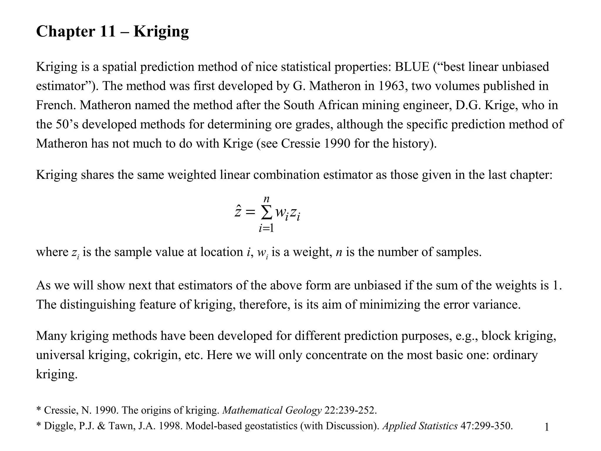
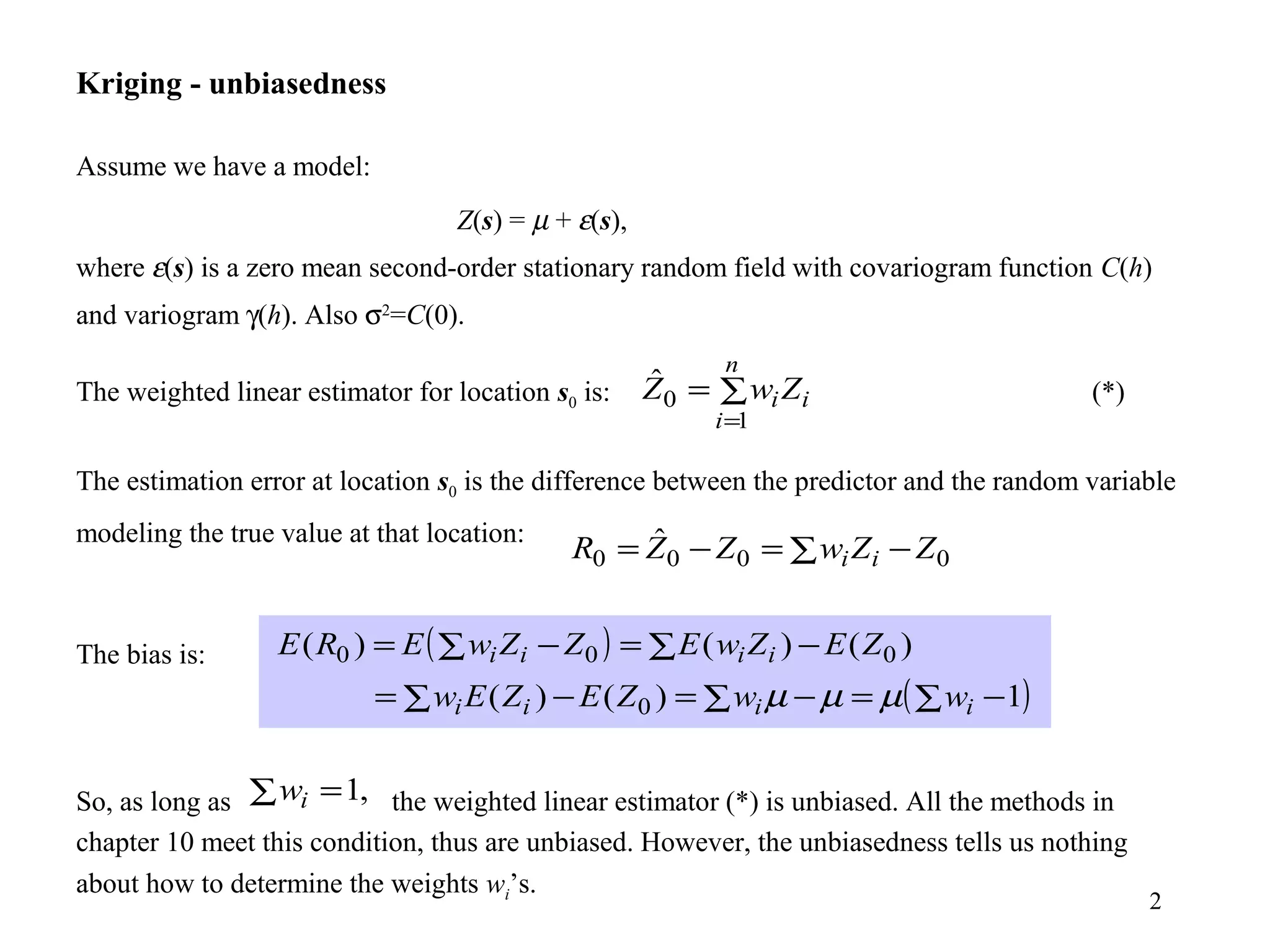
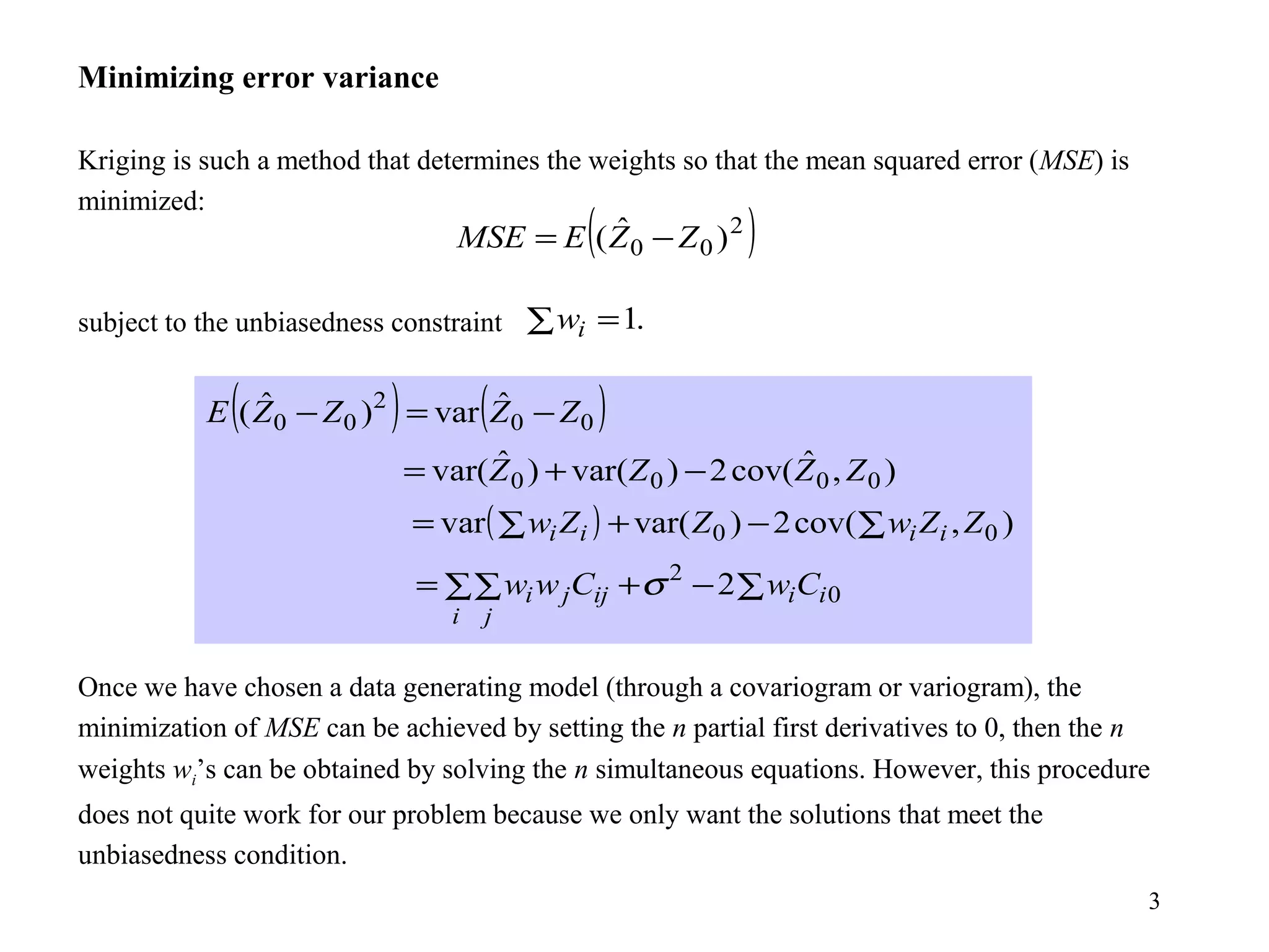
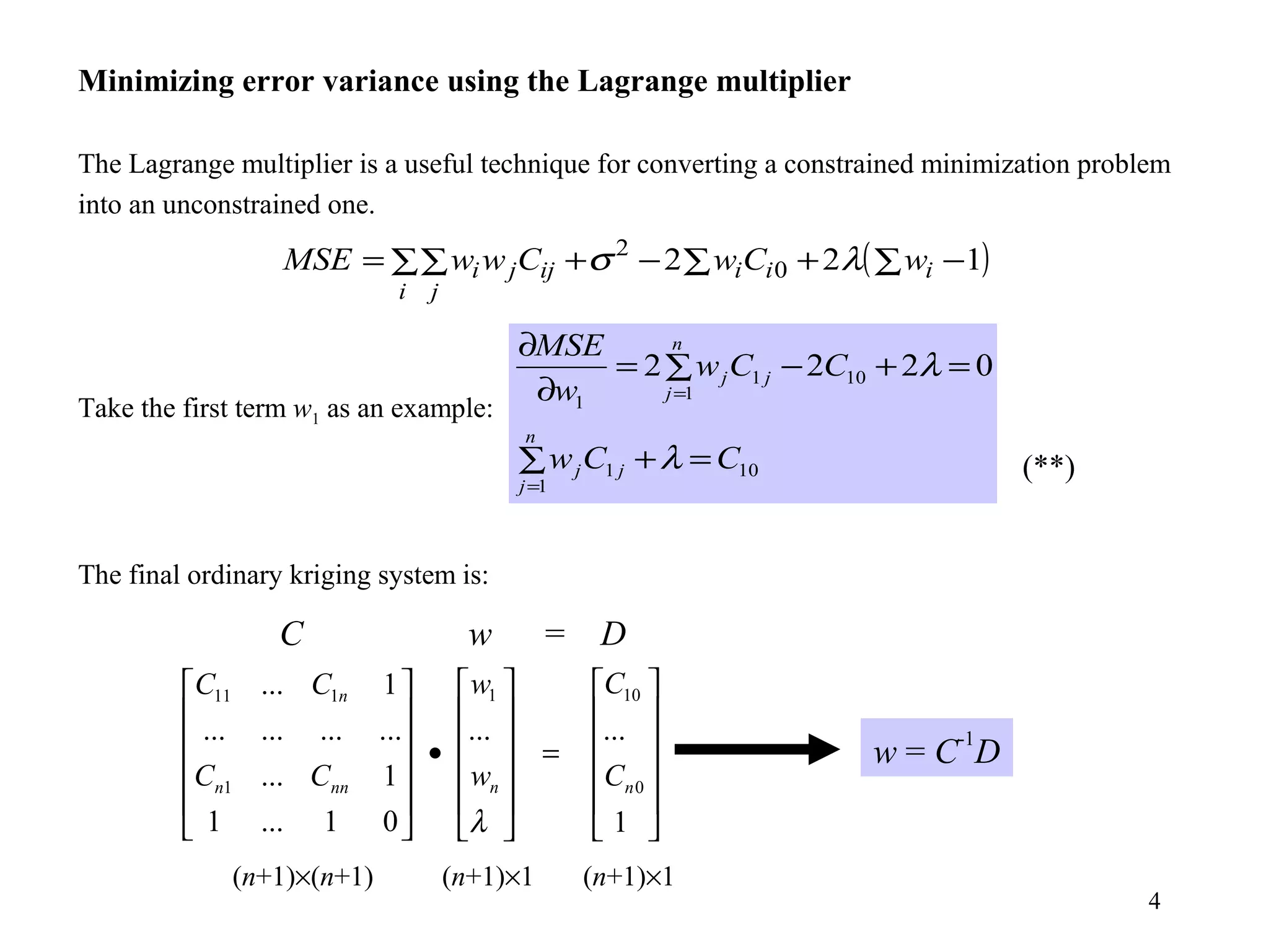
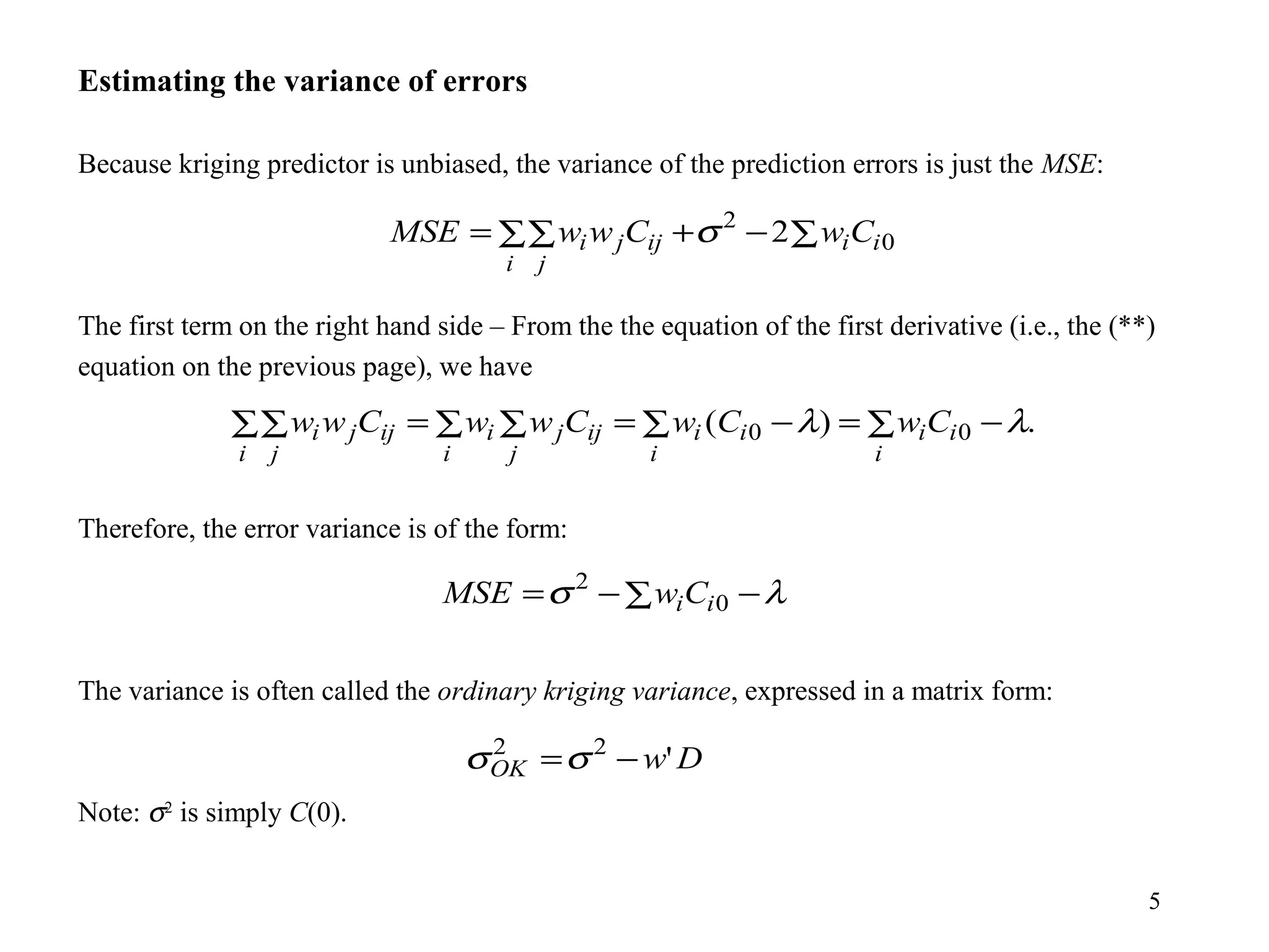
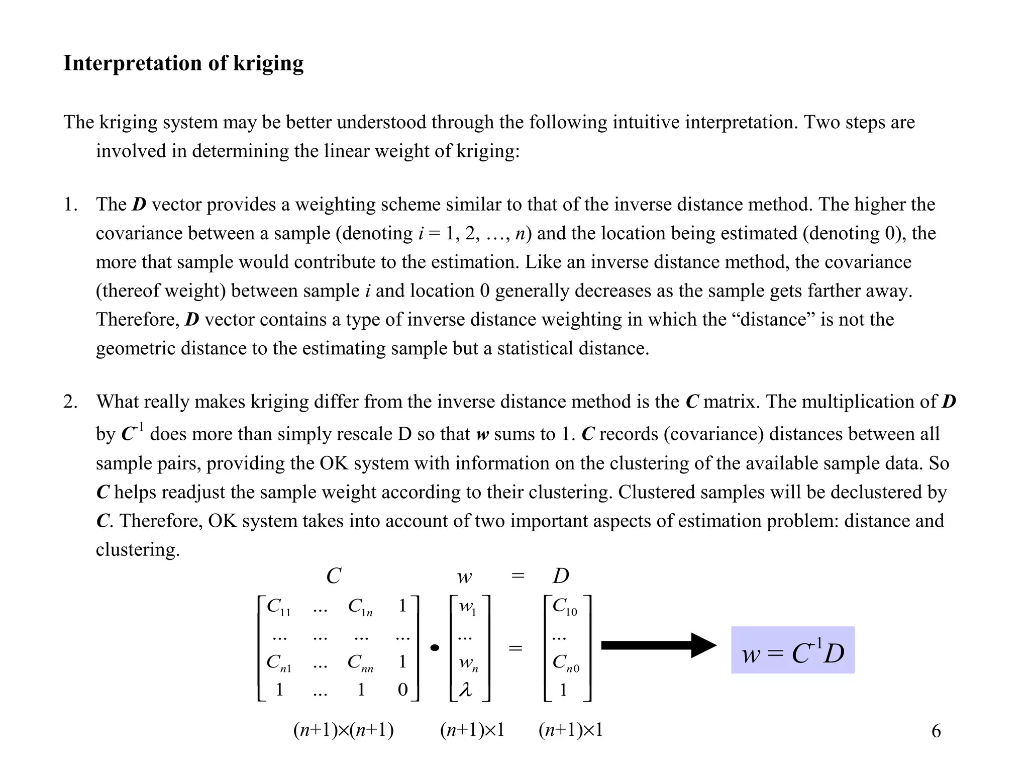
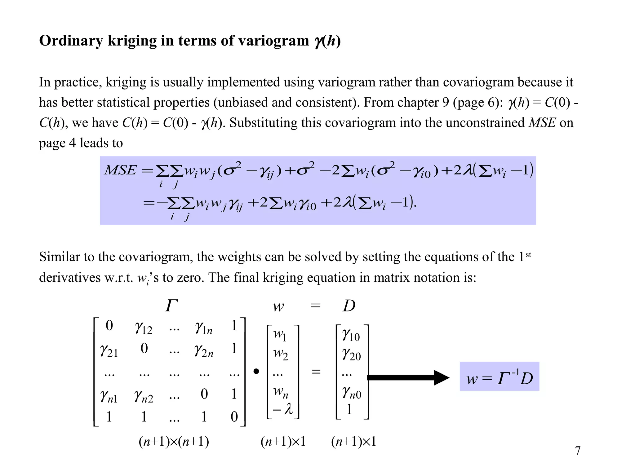
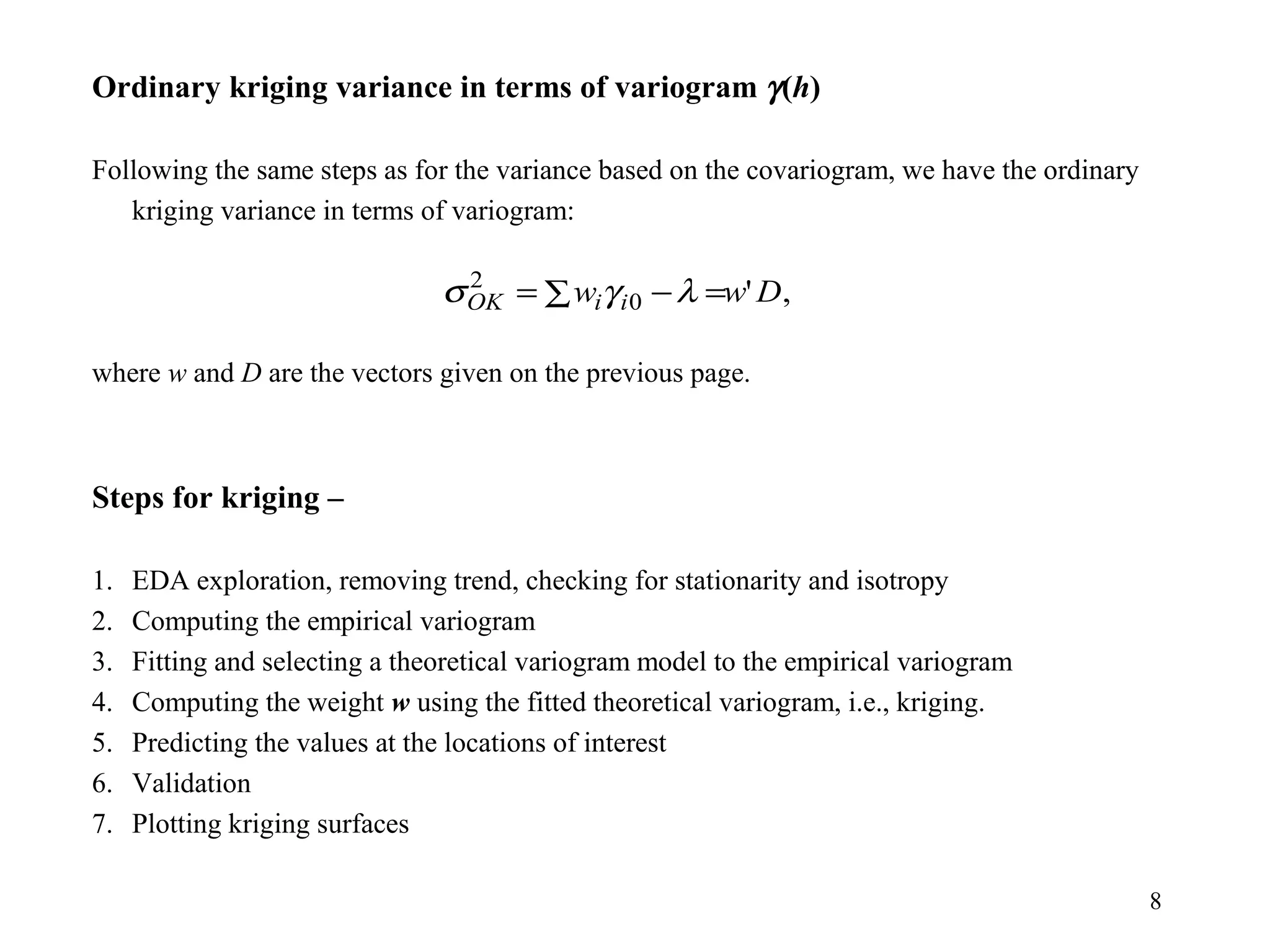
Kriging is a spatial prediction method that provides the "best linear unbiased estimator" (BLUE). It determines weights for a weighted linear combination of sample points that minimizes the prediction error variance. Ordinary kriging focuses on minimizing this error variance based on a variogram model that describes the spatial correlation between sample points. The kriging system is solved to determine the weights, and the predicted values and kriging variance can then be estimated at desired locations.

1. 1
Chapter 11 – Kriging
Kriging is a spatial prediction method of nice statistical properties: BLUE (“best linear unbiased
estimator”). The method was first developed by G. Matheron in 1963, two volumes published in
French. Matheron named the method after the South African mining engineer, D.G. Krige, who in
the 50’s developed methods for determining ore grades, although the specific prediction method of
Matheron has not much to do with Krige (see Cressie 1990 for the history).
Kriging shares the same weighted linear combination estimator as those given in the last chapter:
where zi is the sample value at location i, wi is a weight, n is the number of samples.
As we will show next that estimators of the above form are unbiased if the sum of the weights is 1.
The distinguishing feature of kriging, therefore, is its aim of minimizing the error variance.
Many kriging methods have been developed for different prediction purposes, e.g., block kriging,
universal kriging, cokrigin, etc. Here we will only concentrate on the most basic one: ordinary
kriging.
* Cressie, N. 1990. The origins of kriging. Mathematical Geology 22:239-252.
* Diggle, P.J. & Tawn, J.A. 1998. Model-based geostatistics (with Discussion). Applied Statistics 47:299-350.
∑=
=
n
i
iizwz
1
ˆ

2. 2
Kriging - unbiasedness
Assume we have a model:
Z(s) = µ + ε(s),
where ε(s) is a zero mean second-order stationary random field with covariogram function C(h)
and variogram γ(h). Also σ2
=C(0).
The weighted linear estimator for location s0 is: (*)
The estimation error at location s0 is the difference between the predictor and the random variable
modeling the true value at that location:
The bias is:
So, as long as the weighted linear estimator (*) is unbiased. All the methods in
chapter 10 meet this condition, thus are unbiased. However, the unbiasedness tells us nothing
about how to determine the weights wi’s.
∑=
=
n
i
iiZwZ
1
0
ˆ
∑ −=−= 0000
ˆ ZZwZZR ii
( ) ∑ −=∑ −= )()()( 000 ZEZwEZZwERE iiii
( )∑ −=∑ −=∑ −= 1)()( 0 iiii wwZEZEw µµµ
,1∑ =iw

3. 3
Minimizing error variance
Kriging is such a method that determines the weights so that the mean squared error (MSE) is
minimized:
subject to the unbiasedness constraint
Once we have chosen a data generating model (through a covariogram or variogram), the
minimization of MSE can be achieved by setting the n partial first derivatives to 0, then the n
weights wi’s can be obtained by solving the n simultaneous equations. However, this procedure
does not quite work for our problem because we only want the solutions that meet the
unbiasedness condition.
( )2
00 )ˆ( ZZEMSE −=
.1∑ =iw
( ) ( )00
2
00
ˆvar)ˆ( ZZZZE −=−
),ˆcov(2)var()ˆvar( 0000 ZZZZ −+=
( ) ),cov(2)var(var 00 ZZwZZw iiii ∑−+∑=
0
2
2 ii
i j
ijji CwCww ∑−+∑∑= σ

4. 4
Minimizing error variance using the Lagrange multiplier
The Lagrange multiplier is a useful technique for converting a constrained minimization problem
into an unconstrained one.
Take the first term w1 as an example:
The final ordinary kriging system is:
( )∑ −+∑−+∑∑= 122 0
2
iii
i j
ijji wCwCwwMSE λσ
0222 10
1
1
1
=+−∑=
∂
∂
=
λCCw
w
MSE n
j
jj
10
1
1 CCw
n
j
jj =+∑
=
λ












=












•












1
......
01...1
1...
............
1...
0
101
1
111
nnnnn
n
C
C
w
w
CC
CC
λ
C w = D
(n+1)×(n+1) (n+1)×1 (n+1)×1
w = C
-1
D
(**)

5. 5
Estimating the variance of errors
Because kriging predictor is unbiased, the variance of the prediction errors is just the MSE:
The first term on the right hand side – From the the equation of the first derivative (i.e., the (**)
equation on the previous page), we have
Therefore, the error variance is of the form:
The variance is often called the ordinary kriging variance, expressed in a matrix form:
Note: σ2
is simply C(0).
0
2
2 ii
i j
ijji CwCwwMSE ∑−+∑∑= σ
.)( 00 ∑ −=∑ −=∑ ∑=∑∑
i
ii
i
ii
i j
ijji
i j
ijji CwCwCwwCww λλ
λσ −∑−= 0
2
iiCwMSE
DwOK '22
−=σσ

6. 6
Interpretation of kriging
The kriging system may be better understood through the following intuitive interpretation. Two steps are
involved in determining the linear weight of kriging:
1. The D vector provides a weighting scheme similar to that of the inverse distance method. The higher the
covariance between a sample (denoting i = 1, 2, …, n) and the location being estimated (denoting 0), the
more that sample would contribute to the estimation. Like an inverse distance method, the covariance
(thereof weight) between sample i and location 0 generally decreases as the sample gets farther away.
Therefore, D vector contains a type of inverse distance weighting in which the “distance” is not the
geometric distance to the estimating sample but a statistical distance.
2. What really makes kriging differ from the inverse distance method is the C matrix. The multiplication of D
by C-1
does more than simply rescale D so that w sums to 1. C records (covariance) distances between all
sample pairs, providing the OK system with information on the clustering of the available sample data. So
C helps readjust the sample weight according to their clustering. Clustered samples will be declustered by
C. Therefore, OK system takes into account of two important aspects of estimation problem: distance and
clustering.












=












•












1
......
01...1
1...
............
1...
0
101
1
111
nnnnn
n
C
C
w
w
CC
CC
λ
C w = D
(n+1)×(n+1) (n+1)×1 (n+1)×1
w = C
-1
D

7. 7
Ordinary kriging in terms of variogram γ(h)
In practice, kriging is usually implemented using variogram rather than covariogram because it
has better statistical properties (unbiased and consistent). From chapter 9 (page 6): γ(h) = C(0) -
C(h), we have C(h) = C(0) - γ(h). Substituting this covariogram into the unconstrained MSE on
page 4 leads to
Similar to the covariogram, the weights can be solved by setting the equations of the 1st
derivatives w.r.t. wi’s to zero. The final kriging equation in matrix notation is:
( )∑ −+−∑−+∑∑ −= 12)(2)( 0
222
iii
i j
ijji wwwwMSE λγσσγσ
( ).122 0 ∑ −+∑+∑∑−= iii
i j
ijji wwww λγγ
Γ w = D
(n+1)×(n+1) (n+1)×1 (n+1)×1
w = Γ -1
D














=














−
•
















1
......
01...11
10...
...............
1...0
1...0
0
20
10
2
1
21
221
112
nnnn
n
n
w
w
w
γ
γ
γ
λ
γγ
γγ
γγ

8. 8
Ordinary kriging variance in terms of variogram γ(h)
Following the same steps as for the variance based on the covariogram, we have the ordinary
kriging variance in terms of variogram:
where w and D are the vectors given on the previous page.
Steps for kriging –
1. EDA exploration, removing trend, checking for stationarity and isotropy
2. Computing the empirical variogram
3. Fitting and selecting a theoretical variogram model to the empirical variogram
4. Computing the weight w using the fitted theoretical variogram, i.e., kriging.
5. Predicting the values at the locations of interest
6. Validation
7. Plotting kriging surfaces
,'0
2
Dww iiOK ∑ =−= λγσ

9. 9
Checking and removing trends (make the data stationary)
Example: soil pH value in the Gigante plot of Panama, using the full data set (soil.dat, has 349 data
points).
The data appear to have a trend in the northwest-southeastern direction. To remove such a trend, we
fit the data using using model: z = 5.67 - 0.003295x + 0.001025y + 4.521e-6x2
+ ε. Terms y2
and x×y
are not significant. It seems that the trend surface analysis has detrended the data.
0 100 200 300 400 500
0200400600800
0 100 200 300 400 5000200400600800
Before detrended After detrended
High
Low

10. 10
Has the trend really been removed?
We further check it using variograms. The comparison of the variograms before and after detrending
confirms that there is no trend in the residuals. We are confident that the residuals of the trend surface
analysis are likely stationary. We can now go on to do kriging.
>soil.geodat=as.geodata(soil.dat,coords.col=2:3,data.col=5,borders=T)
>variog.b0=variog(soil.geodat,uvec=seq(0,500,by=5), max.dist=500)
>plot(variog.b0)
>variog.b2=variog(soil.geodat,uvec=seq(0,500,by=5),trend="2nd",max.dist=500)
>plot(variog.b2)

11. 11
Spherical model
Logistic model
Fitting a variogram
Several variogram models can be fitted to the data. For illustration purpose, only two models
(the spherical and logistic models) are shown here. By visual inspection, it seems that the
logistic model may capture the spatial autocorrelation better than the spherical model,
particularly at short distance lag. However, the sigmoid shape of the logistic model may not
reflect the intrinsic feature of the data. We will use the spherical model for kriging.
2
2
0009258.0
0001072.0
1065.0)(
h
h
h +=γ
Logistic model:

12. 12
R implementation using geoR- ordinary kriging
1. Compute variogram by directly considering trend (i.e., removing 2nd
order trend. Kriging will
automatically put back the trend in the final prediction):
>variog.b2=variog(soil.geodat,uvec=seq(0,500,by=5),trend="2nd",max.dist=500)
2. Model variogram using spheric variogram model:
>pH.sph=variofit(variog.b2,cov.model="spherical")
>pH.sph # also try summary(pH.sph) to see the output
variofit: model parameters estimated by WLS (weighted least squares):
covariance model is: spherical
parameter estimates:
tausq sigmasq phi
0.1240 0.0955 130.7104
3. Fitting logistic model:
> u=variog.b2$u;v=variog.b2$v
> logist.nls=nls(v~c0+a*u^2/(1+b*u^2),start=c(c0=0.05,a=0.25,b=0.1))
>logist.nls
model: y ~ c0 + a * x^2/(1 + b * x^2)
data: parent.frame()
c0 a b
0.1064792 0.0001072 0.0009258
residual sum-of-squares: 0.04605
nugget (c0) c1 range
for 0 < h ≤ 130.71
for h ≥ 130.71






−+= 3
)
71.130
(
2
1
71.1302
3
0955.01240.0)(
hh
hγ
0955.01240.0)( +=hγ
2
2
0009258.0
0001072.0
1065.0)(
h
h
h +=γ
Logistic model:

13. 13
R implementation - ordinary kriging
1. Generate locations at which interpolation is needed:
>x=soil.dat$gx; y=soil.dat$gy
>prd.loc=expand.grid(x=sort(unique(x)),y=sort(unique(y)))
2. Run krige.conv for spatial interpolation:
>pH.prd=krige.conv(soil.geodat,loc=prd.loc,krige=krige.control(cov.model="spherical",cov.pars
=c(0.09549404,130.71043698)))
3. View the prediction: You can directly apply image to pH.prd.
Here we want to have more control over the features of the image,
We create matrix for the pH.prd$predict and then apply image:
>pH.prd.mat=matrix(pH.prd$predict,byrow=T,ncol=84)
>image(unique(prd.loc$x),unique(prd.loc$y),t(pH.prd.mat),
xlim=c(-20,500),ylim=c(-20,820),xlab="x",ylab="y")
>lines(gigante.border,lwd=2,col=“green”)
>contour(pH.prd,add=T)
We can do the same thing to view the variation in the prediction:
pH.prd$krige.var. Taking the squared root, it is prd.se.
>pH.prd.se.mat=matrix(sqrt(pH.prd$krige.var),
byrow=T,ncol=84)
>image(unique(prd.loc$x),unique(prd.loc$y),t(pH.prd.se.mat),
xlim=c(-20,500),ylim=c(-20,820),xlab="x",ylab="y")
>lines(gigante.border,lwd=2)

14. 14
Plot prediction variance
It is desirable to view the variation of the prediction: pH.prd$krige.var. Taking the squared root for
prd.se.
>pH.prd.se.mat=matrix(sqrt(pH.prd$krige.var),byrow=T,ncol=84)
>image(unique(prd.loc$x),unique(prd.loc$y),t(pH.prd.se.mat),xlim=c(-20,500),
ylim=c(-20,820),xlab="x",ylab="y")
>lines(gigante.border,lwd=2,col="blue")
>contour(unique(prd.loc$x),unique(prd.loc$y),t(pH.prd.se.mat),xlim=c(-20,500),
ylim=c(-20,820),add=T)
pH surface pH std error surface pH std error with contour

15. 15
1. Independent data validation:
Compare the predicted with the observed
data. As shown in the left table, these 13
data samples were not included in the
kriging analysis. The predictions were
generated from:
>pH.prd13=krige.conv(soil.geodat,loc=
prd.loc13,krige=krige.control(cov.model=
"spherical",cov.pars=c(0.09549,130.71043)))
2. Cross-validation:
Deleting one observation each time from
the data set and then predicting the deleted
observation using the remaining
observations in the data set. This process is
repeated for all observations. Residuals are
then analyzed using standard techniques of
regression analysis to check the underlying
model assumptions.
Evaluating the outputs
of kriging prediction:
SrfID gx gy Site pH pred var se.fit
31 240 8 site8mN 4.92 4.304 0.0088 0.0936
123 240 232 site8mS 5.97 5.933 0.0109 0.1046
124 240 220 site20mS 5.57 5.762 0.0203 0.1426
128 300 260 site20mN 5.41 5.375 0.0198 0.1406
190 358 420 site2mW 5.28 5.268 0.0033 0.0573
242 362 540 site2mE 5.23 5.437 0.0039 0.0627
243 368 540 site8mE 5.04 5.343 0.0104 0.1020
290 238 600 site2mW 4.63 5.086 0.0042 0.0647
291 232 600 site8mW 5.45 5.177 0.0145 0.1202
292 220 600 site20mW 5.4 5.371 0.0254 0.1595
310 422 660 site2mE 5.33 5.545 0.0033 0.0573
312 440 660 site20mE 6.17 5.747 0.0185 0.1361
360 478.6 538.6 site2mSW 5.55 5.310 0.0033 0.0572

16. 16
Block kriging
In many occasions, we are interested in estimating the value in a block (cell) rather than that
at a point. The block kriging system is similar to that of the
OK, of the form:
where i.e., the covariogram between
block A and sample point i is the average of the covariograms between the points
locating within A and i.
The block kriging variance is: where
+
+
+
+
+
+
Block A
. .
. .
+ observed samples
. regularly spaced locations
set up within the block












=












•












1
......
01...1
1...
............
1...
11
1
111
nA
A
nnnn
n
C
C
w
w
CC
CC
λ
C w = D
(n+1)×(n+1) (n+1)×1 (n+1)×1
,
1
∑=
∈Aj
ijiA C
A
C
,'2
DwCAAOK −=σ .
1
2 ∑ ∑=
∈ ∈Ai Aj
ijAA C
A
C

17. 17
R implementation - block kriging
Block kriging is achieved by using OK:
1. Create a systematical grid lattice (as dense as you want) using expand.grid.
2. Use krige.conv for OK to do spatial interpolation for the grids.
3. Average the values of those grids falling within the defined block.
+
+
+
+
+
+
Block A
. .
. .
+ observed samples
. regularly spaced locations
set up within the block

18. 18
Spatial estimation: additive/nonadditive variables
Some precaution is necessary before applying geostatistical analysis to your data. The method
does not universally apply to any type of data.
Additive variable:
Nonadditive variable:
Nonadditive variables include: number of species in a block, ratio data (e.g., number of cars
per household in a city block). Geostatistics is invalid for analyzing nonadditive variables
because subtraction makes no sense here.
5 balls 3
7 4
8
11
scaled up
3 colors
(1b, 2r, 2 w)
5 colors
4 colors
scaled up
3 colors
(1b, 1g, 1y)
1 color
(4g)
3 colors
(3b, 2r, 2 w)

19. 19
Spatial estimation: scale effect
Few spatial data (point process is an exception) can avoid the problem of the size of sample area
(called support in geostat, or modifiable areal unit in geography, or grain size in landscape
ecology).
In many practical applications, the support of the samples is not the same as the support of the
estimates we are trying to calculate. For example, when assessing gold ore grades in an area, we
take samples from drill hole cores, but in mining operation we treat truckloads as the size of
sample (consider a truckload either as ore or as waste).
So a critical and difficult question is: can we infer about the properties of a variable at different
levels of supports from the observations sampled at a particular support? In other words, can we
scale down or up a spatial process?
0 1 2 3 4
010203040
rg am m a(100, 1)
0 2 4 6 8
0510152025
rg am m a(100, 3)
?

20. 20
Grain
size (m)
No. stems/m2
(std. error)
No. species/m2
(std. error)
5×5 0.671 (0.244) 0.585 (0.197)
10×10 0.671 (0.167) 0.475 (0.095)
20×20 0.671(0.130) 0.318 (0.038)
25×25 0.671 (0.121) 0.267 (0.026)
50×50 0.671 (0.100) 0.129 (0.008)
100×100 0.671 (0.085) 0.049 (0.001)
250×250 0.671 (0.048) 0.011 (0.0004)
500×500 0.671 (0.041) 0.003 (< 0.001)
500×1000 0.671 0.0016
Spatial estimation: scale effect
Number of stems and number of species per
m2
at different sampling scales (grain size) in
a 1000×500 m rain forest of Malaysia. The
entire plot has 335,356 trees belonging to 814
species. The densities at each grain size were
computed as follows: (1) divide the plot into a
grid system using a given scale (e.g., 5×5 m),
(2) count the total number of stems and the
number of species in each cells, respectively,
(3) average these two quantities across all the
cells, and (4) then divide the averages by the
scale.
The results clearly show how sampling scale
profoundly affects the species diversity. They
suggest that diversity based on per unit area
(the last column) is a misleading measurement
for comparing diversity between two
ecosystems.

21. 21
Spatial estimation: scale effect
“This problem of the discrepancy between the support of our samples and the
intended support of our estimates is one of the most difficult we face in
estimation.”
Isaaks & Srivastava (1989, page 193)