Downloaded 33 times

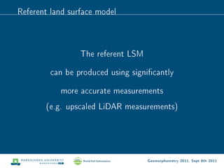
![Example
library(maptools); library(gstat); library(rgdal)
# Download the datasets:
data.url - http://geomorphometry.org/system/files/GDEM_assessment.zip
download.file(data.url, destfile=GDEM_assessment.zip)
unzip(GDEM_assessment.zip)
...
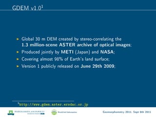
str(grid.list[[j]]@data)
'data.frame': 15000 obs. of 2 variables:
$ zlatibor_LDEM: num 1010 1010 1008 1007 1005 ...
$ zlatibor_GDEM: num 997 1000 1000 1000 998 ...
Geomorphometry 2011, Sept 8th 2011](https://image.slidesharecdn.com/ovhenglgeomorphometry2011-110904075007-phpapp01/85/A-statistical-assessment-of-GDEM-using-LiDAR-data-20-320.jpg)
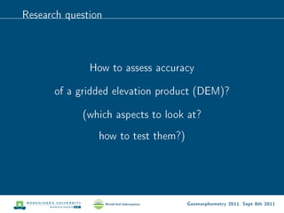
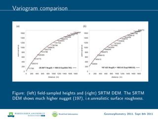
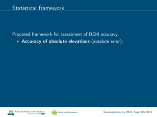
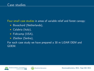
![Variogram comparison (Calabria)
vgm_LDEM.list[[2]]
model psill range kappa
1 Nug 75.14568 0.000 0.0
2 Mat 150391.85522 2624.796 1.2
vgm_GDEM.list[[2]]
model psill range kappa
1 Nug 18.55683 0.000 0.0
2 Mat 199978.44320 3184.624 1.2
Geomorphometry 2011, Sept 8th 2011](https://image.slidesharecdn.com/ovhenglgeomorphometry2011-110904075007-phpapp01/85/A-statistical-assessment-of-GDEM-using-LiDAR-data-25-320.jpg)
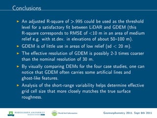

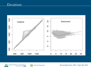
This document presents a statistical assessment of the accuracy of the Global Digital Elevation Model (GDEM) using LiDAR data. It proposes a framework to evaluate GDEM accuracy by assessing absolute elevation errors, positional accuracy of hydrological features, surface roughness representation, and user satisfaction. Case studies in four areas show regression models can evaluate elevation fit, with an R-squared value above 0.995 indicating satisfactory accuracy for GDEM in areas of medium relief. The document concludes GDEM has little usefulness in areas of low relief.


![Heritage hetherington lidar_pdf[1]](https://cdn.slidesharecdn.com/ss_thumbnails/heritagehetheringtonlidarpdf1-100701210824-phpapp02-thumbnail.jpg?width=640&height=640&fit=bounds)


