Download as PDF, PPTX
![Hierarchical statistical modeling (HM)
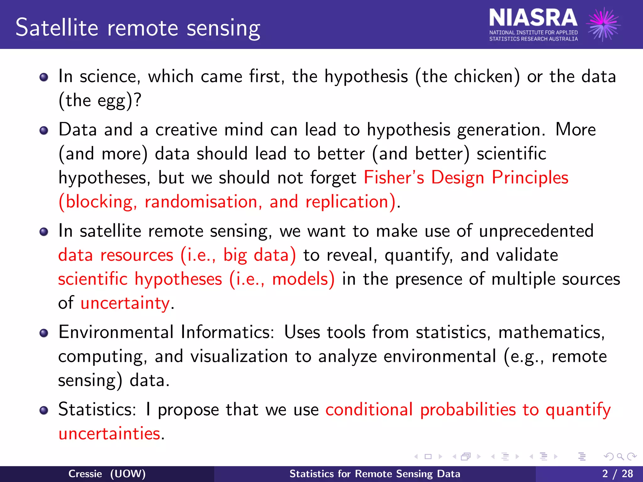
Step away from remote sensing for the moment to get a broader
perspective on uncertainty quantification in science.
Let Y be the data, X be the process (or state) of interest, and θ be
unknown parameters. (For example, in my research in spatio-temporal
statistics, Y might have dimension 106 − 109, X might be of the
same order, and θ might have dimension 102 − 104.)
[A|B] denotes the conditional distribution of generic quantity A, given
generic quantity B; and [B] denotes the distribution of B.
[A,B] denotes the joint distribution of A and B. Then
[A,B] = [A|B] · [B].
Cressie (UOW) Statistics for Remote Sensing Data 9 / 28](https://image.slidesharecdn.com/cressiebirdseyeviewofstatistics-170827232447/75/Program-on-Mathematical-and-Statistical-Methods-for-Climate-and-the-Earth-System-Opening-Workshop-A-Bird-s-Eye-View-of-Statistics-for-Remote-Sensing-Data-Noel-Cressie-Aug-22-2017-9-2048.jpg)
![HM captures sources of uncertainty
Sources of uncertainty: the data, the process, and the parameters.
All uncertainties can be expressed through the joint distribution,
[Y , X, θ]. From the previous slide,
[Y , X, θ] = [Y , X|θ] · [θ]
= [Y |X, θ] · [X|θ] · [θ]
Data model: [Y |X, θ]
Process model: [X|θ]
Parameter model: [θ]
Inference is on X (and θ) through the posterior distribution,
[X, θ|Y ] = [Y |X, θ][X|θ][θ]/[Y ].
This is known as Baye’s Rule, and it relies on knowing the normalizing
constant, [Y ]. An alternative strategy is to simulate from [X, θ|Y ].
Cressie (UOW) Statistics for Remote Sensing Data 10 / 28](https://image.slidesharecdn.com/cressiebirdseyeviewofstatistics-170827232447/75/Program-on-Mathematical-and-Statistical-Methods-for-Climate-and-the-Earth-System-Opening-Workshop-A-Bird-s-Eye-View-of-Statistics-for-Remote-Sensing-Data-Noel-Cressie-Aug-22-2017-10-2048.jpg)
![Predictive distribution
As a concept, the predictive distribution is different from the posterior
distribution. In words, it is the conditional distribution of the process X
given the data Y . What about θ?
Three cases:
0 θ is known, and hence the parameter model is degenerate at θ. The
posterior distribution is [X|Y , θ] – since θ is known, this is also the
predictive distribution.
1 θ is fixed but unknown, and it is estimated from the data Y ; call the
estimate θ. The parameter model is assumed degenerate at θ, and the
(empirical) predictive distribution is [X|Y , θ].
2 θ is unknown, and its uncertainty is captured with the parameter model
[θ]. The posterior distribution is [X, θ|Y ], and the predictive
distribution is [X|Y ], after marginalizing over θ.
Case 0 is often unrealistic; Case 1 is called empirical hierarchical
modeling (EHM); and Case 2 is called Bayesian hierarchical modeling
(BHM).
Cressie (UOW) Statistics for Remote Sensing Data 11 / 28](https://image.slidesharecdn.com/cressiebirdseyeviewofstatistics-170827232447/75/Program-on-Mathematical-and-Statistical-Methods-for-Climate-and-the-Earth-System-Opening-Workshop-A-Bird-s-Eye-View-of-Statistics-for-Remote-Sensing-Data-Noel-Cressie-Aug-22-2017-11-2048.jpg)
![States of knowledge of θ
The three cases can be defined in terms of “states of knowledge” on θ.
Case 0: θ is known; often an unrealistic state of knowledge.
Case 1: θ is fixed but unknown; classical frequentist state of
knowledge of θ. This results in empirical hierarchical modeling
(EHM).
Case 2: θ is unknown and has probability distribution [θ]; Bayesian
state of knowledge of θ. This results in Bayesian hierarchical
modeling (BHM).
Cressie (UOW) Statistics for Remote Sensing Data 12 / 28](https://image.slidesharecdn.com/cressiebirdseyeviewofstatistics-170827232447/75/Program-on-Mathematical-and-Statistical-Methods-for-Climate-and-the-Earth-System-Opening-Workshop-A-Bird-s-Eye-View-of-Statistics-for-Remote-Sensing-Data-Noel-Cressie-Aug-22-2017-12-2048.jpg)
![Inference on the state X
Since X is uncertain, it is modeled as a random quantity. Inference on
a random quantity is sometimes called “prediction.” This explains the
terminology, predictive distribution; for the three cases, it is:
Case 0: [X|Y , θ] = [Y |X, θ] · [X|θ]/[Y |θ]
Case 1: [X|Y , θ] = [Y |X, θ] · [X|θ]/[Y |θ],
Case 2: [X|Y ] = [Y |X, θ] · [X|θ] · [θ]dθ/[Y ],
and it is not always the same as the posterior distribution.
Inference on X should be based on the predictive distribution. This is
fundamental to Uncertainty Quantification (UQ)!
In remote sensing, each footprint has an X. Typically, the retrieved
state ˆX is the mode of the predictive distribution; to my knowledge,
only Case 0 or Case 1 have been considered in the literature.
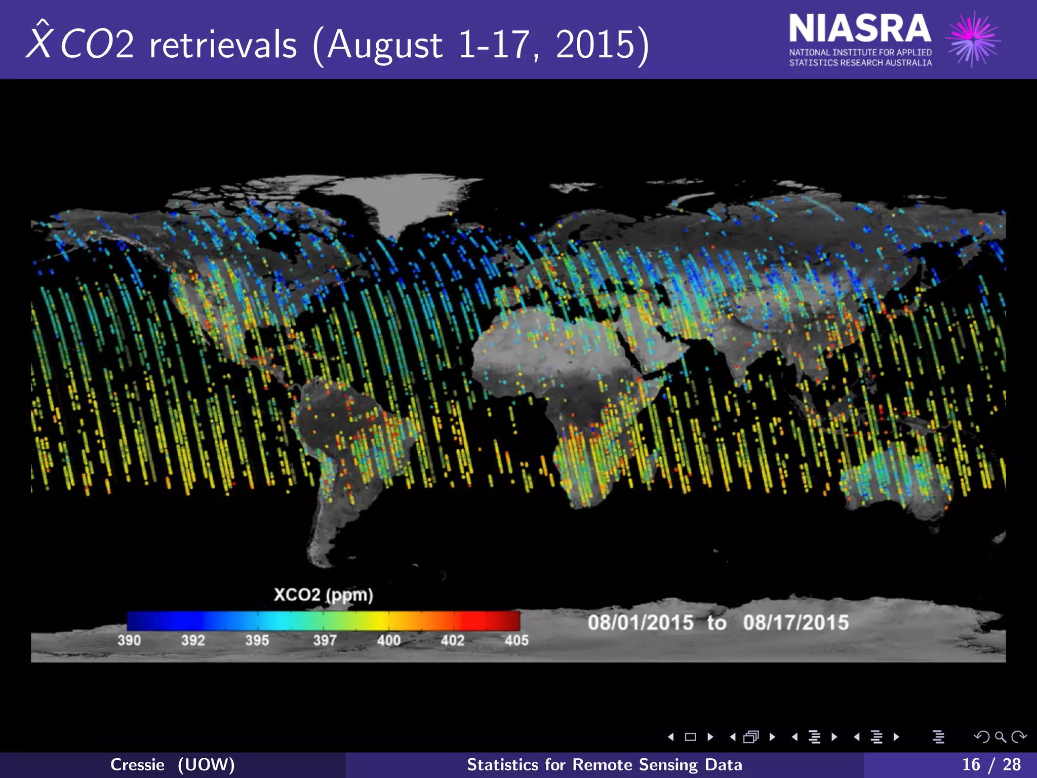
XCO2 is the average CO2 (in ppm) in the atmospheric column with
base given by the footprint; ˆXCO2 is its prediction obtained from the
predictive distribution of X given Y.
Cressie (UOW) Statistics for Remote Sensing Data 13 / 28](https://image.slidesharecdn.com/cressiebirdseyeviewofstatistics-170827232447/75/Program-on-Mathematical-and-Statistical-Methods-for-Climate-and-the-Earth-System-Opening-Workshop-A-Bird-s-Eye-View-of-Statistics-for-Remote-Sensing-Data-Noel-Cressie-Aug-22-2017-13-2048.jpg)
![Predictive distribution, ctd
There is often too much information in [X|Y ], which is a (possibly
high-dimensional) probability distribution.
The predictive mean and predictive variance (equivalently, predictive
covariance for multivariate X) are often chosen as summaries of the
predictive distribution:
E(X|Y ) = X[X|Y ]dX
var(X|Y ) = XXT
[X|Y ]dX − E(X|Y )E(X|Y )T
.
Cressie (UOW) Statistics for Remote Sensing Data 17 / 28](https://image.slidesharecdn.com/cressiebirdseyeviewofstatistics-170827232447/75/Program-on-Mathematical-and-Statistical-Methods-for-Climate-and-the-Earth-System-Opening-Workshop-A-Bird-s-Eye-View-of-Statistics-for-Remote-Sensing-Data-Noel-Cressie-Aug-22-2017-17-2048.jpg)
![Predictive distribution, ctd
If X1, . . . , XK is a sample from the predictive distribution [X|Y ], then:
E(X|Y )
1
K
K
k=1
Xk ≡ XK ,
and
var(X|Y )
1
K
K
k=1
XkXT
k − XK X
T
K ≡ CK .
As mentioned above, the predictive mode:
mode(X|Y ) ≡ arg max
X
[X|Y ] ,
is a summary that is often chosen in satellite missions.
Twenty-first-century strategy: Learn how to sample X1, . . . , XK from
the predictive distribution, [X|Y ], and approximate any summary of it
for K large.
Cressie (UOW) Statistics for Remote Sensing Data 18 / 28](https://image.slidesharecdn.com/cressiebirdseyeviewofstatistics-170827232447/75/Program-on-Mathematical-and-Statistical-Methods-for-Climate-and-the-Earth-System-Opening-Workshop-A-Bird-s-Eye-View-of-Statistics-for-Remote-Sensing-Data-Noel-Cressie-Aug-22-2017-18-2048.jpg)
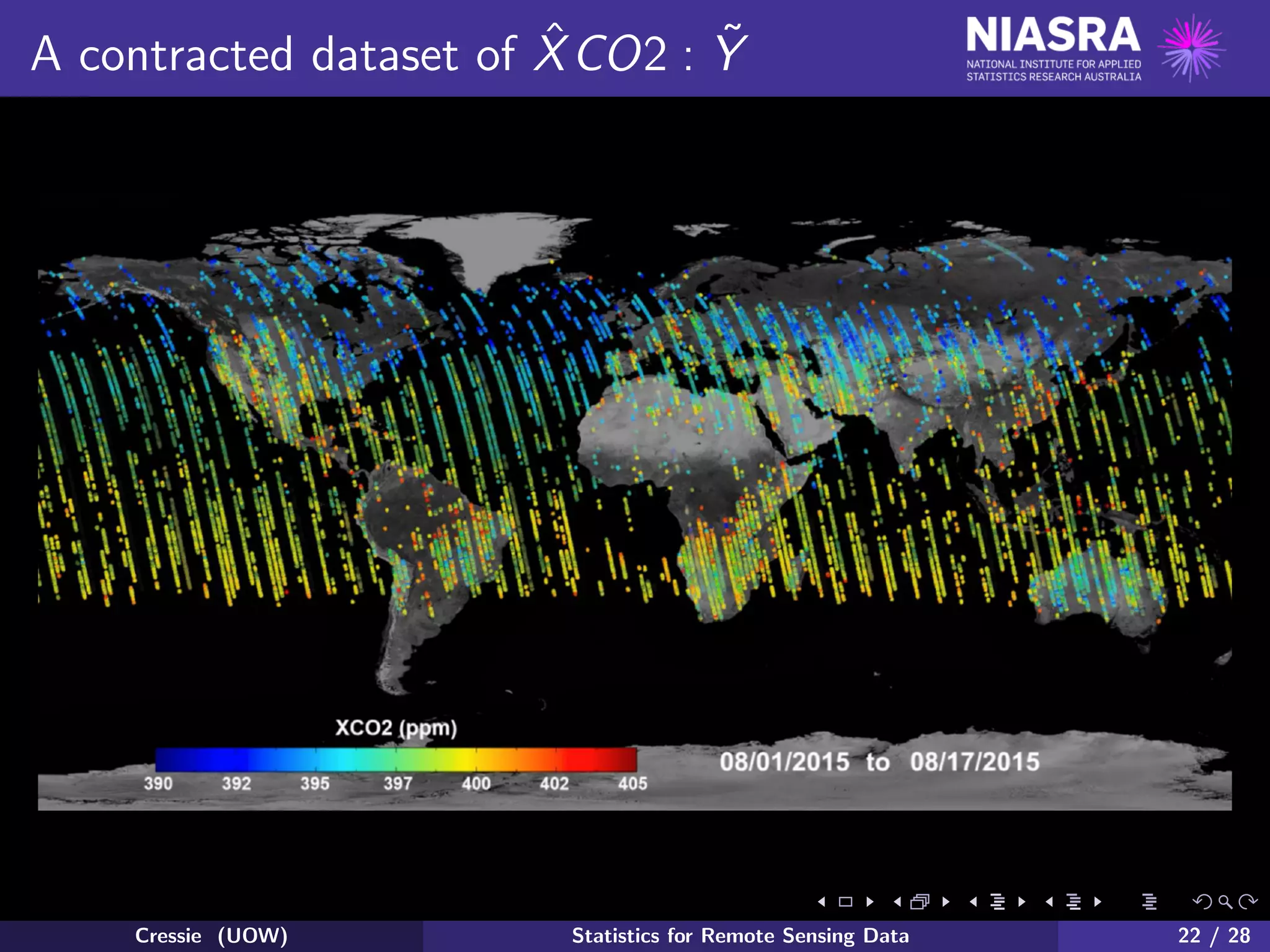
![Satellite remote sensing, revisited (3)
At the next level, called Level 2, OCO-2 focuses on inferring not the
four-dimensional field X, but the contracted set of state values:
X ≡ {XCO2(xi , yi ; ti ) : i = 1, · · · , n},
where formally the XCO2 field is:
XCO2(x, y; t) ≡
1
Psurf (x, y)
Psurf (x,y)
0
X(x, y, h; t)dh .
If [X|θ] = n
i=1[XCO2(xi , yi ; ti )|θ] (i.e., if there is statistical
independence within X), then
[X|Y , θ] =
n
i=1
{[XCO2(xi , yi ; ti )|XCO2(xi , yi ; ti ), θ]·[XCO2(xi , yi ; ti )|θ]},
and it is appropriate that inference proceeds on a
sounding-by-sounding basis. Is the independence assumption
reasonable?
Cressie (UOW) Statistics for Remote Sensing Data 23 / 28](https://image.slidesharecdn.com/cressiebirdseyeviewofstatistics-170827232447/75/Program-on-Mathematical-and-Statistical-Methods-for-Climate-and-the-Earth-System-Opening-Workshop-A-Bird-s-Eye-View-of-Statistics-for-Remote-Sensing-Data-Noel-Cressie-Aug-22-2017-23-2048.jpg)
![Satellite remote sensing, revisited (4)
Because of atmospheric transport of CO2, the four-dimensional field
X is spatio-temporally dependent. Then the three-dimensional field,
XCO2 ≡ {XCO2(x, y; t) : (x, y) ∈ Dg , t ∈ Dt},
is also spatio-temporally dependent. Recall that X consists of just n
values of XCO2.
Since XCO2 is spatio-temporally dependent, so too is ˜X. Then
[X|θ] =
n
i=1
[XCO2(xi , yi ; ti )|θ],
and hence inference on X, or XCO2, or X, should not proceed on a
sounding-by-sounding basis. But it does!
Cressie (UOW) Statistics for Remote Sensing Data 24 / 28](https://image.slidesharecdn.com/cressiebirdseyeviewofstatistics-170827232447/75/Program-on-Mathematical-and-Statistical-Methods-for-Climate-and-the-Earth-System-Opening-Workshop-A-Bird-s-Eye-View-of-Statistics-for-Remote-Sensing-Data-Noel-Cressie-Aug-22-2017-24-2048.jpg)
![Satellite Remote Sensing, Revisited (5)
Sounding-by-sounding retrievals are almost ubiquitous in satellite remote
sensing. Given this, how should Uncertainty Quantification proceed?
The data are Y ; OCO-2 “smooths” or “processes” them, and the
estimate of ˜X is
Y = {XCO2(xi , yi , ; ti ) : i = 1, · · · , n} .
I suggest we do something different. By contracting and marginalizing
[X|Y , θ], the predictive distribution, [ ˜X|Y , θ], can be obtained.
Consequently, the retrieval, ˆXCO2(xi , yi ; ti ), should be obtained from
all Y , not just Y(xi , yi ; ti ). This is sometimes called a joint retrieval,
but I have never seen it actually done.
Cressie (UOW) Statistics for Remote Sensing Data 25 / 28](https://image.slidesharecdn.com/cressiebirdseyeviewofstatistics-170827232447/75/Program-on-Mathematical-and-Statistical-Methods-for-Climate-and-the-Earth-System-Opening-Workshop-A-Bird-s-Eye-View-of-Statistics-for-Remote-Sensing-Data-Noel-Cressie-Aug-22-2017-25-2048.jpg)
![Satellite Remote Sensing, Revisited (6)
We want to make inference on the CO2 field X, or its surface
derivative, XF , the surface-flux field. Then the predictive distribution
for data Y is:
[X|Y , θ] ∝ [Y |X, θ] · [X|θ].
If we use data Y (i.e., the XCO2 values), then we should build the
conditional probability models, [Y |X, θ], [X|θ] (and eventually worry
about θ). Notice that the process model, [X|θ], has not changed.
We need to build the spatio-temporal process model [X|θ]. A
geostatistical model that involves atmospheric transport is one choice;
a spatio-temporal random effects (SRE) model is another choice.
Recall XCO2 and XF . Inference on XCO2 is called Level 3
estimation, and inference on XF is called Level 4 estimation.
Cressie (UOW) Statistics for Remote Sensing Data 26 / 28](https://image.slidesharecdn.com/cressiebirdseyeviewofstatistics-170827232447/75/Program-on-Mathematical-and-Statistical-Methods-for-Climate-and-the-Earth-System-Opening-Workshop-A-Bird-s-Eye-View-of-Statistics-for-Remote-Sensing-Data-Noel-Cressie-Aug-22-2017-26-2048.jpg)
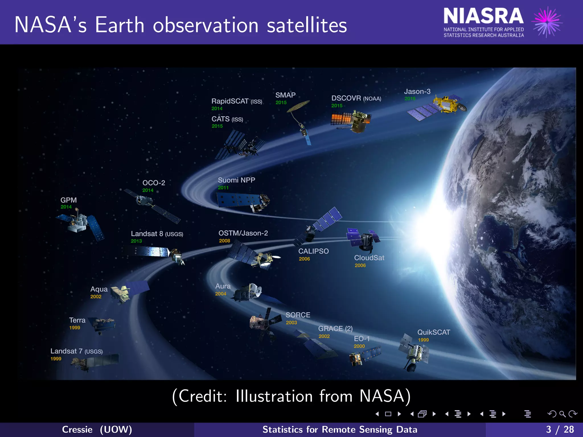
This document outlines the use of statistical methodologies in the analysis and interpretation of remote sensing data, specifically focusing on NASA's OCO-2 satellite for measuring atmospheric CO2 levels. It discusses hierarchical statistical modeling to quantify uncertainties, the importance of Bayesian principles, and the predictive distribution as it pertains to atmospheric data. The document emphasizes the need for joint retrieval approaches to enhance the accuracy of CO2 field inference and improve carbon-cycle knowledge.