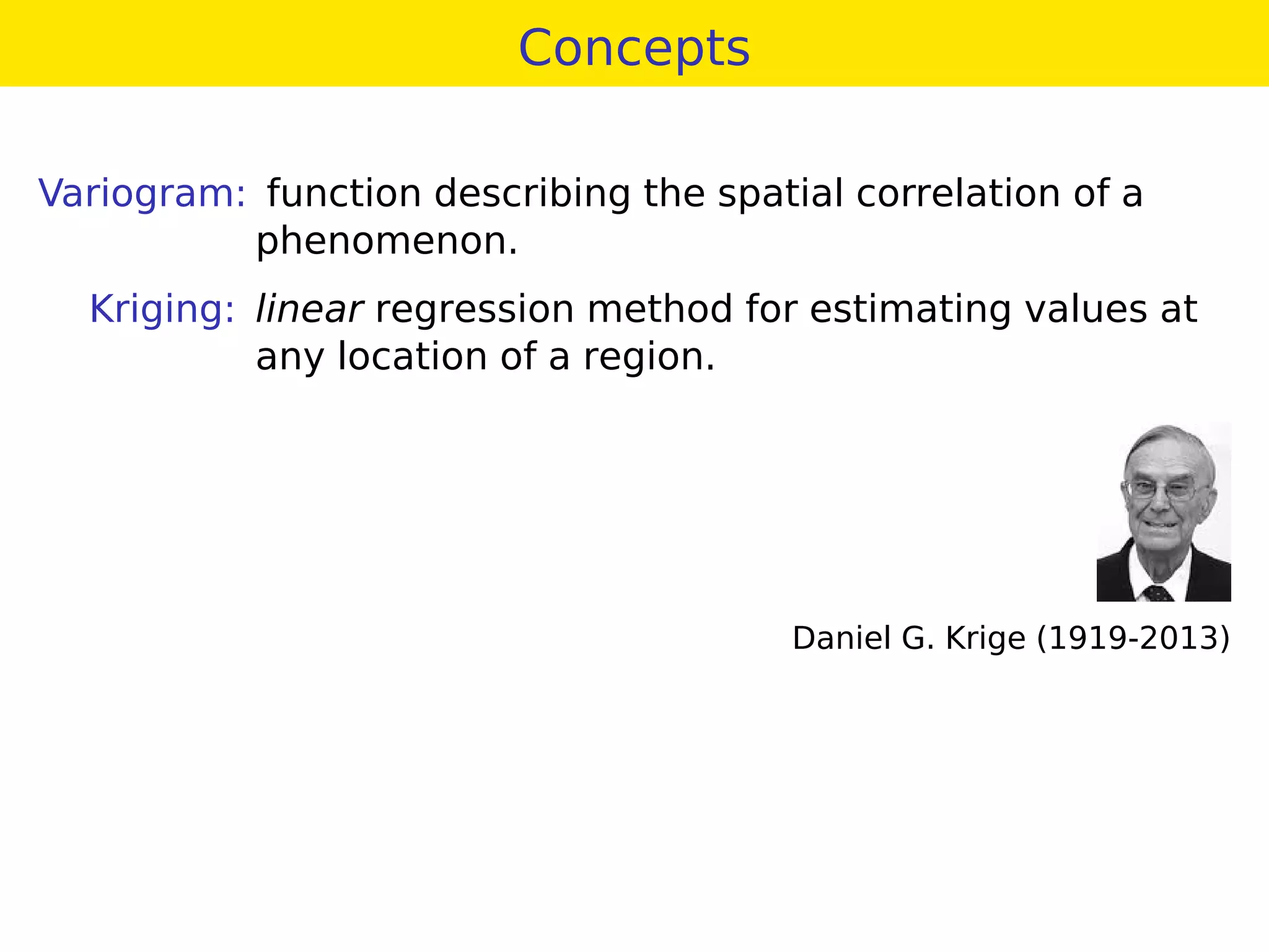
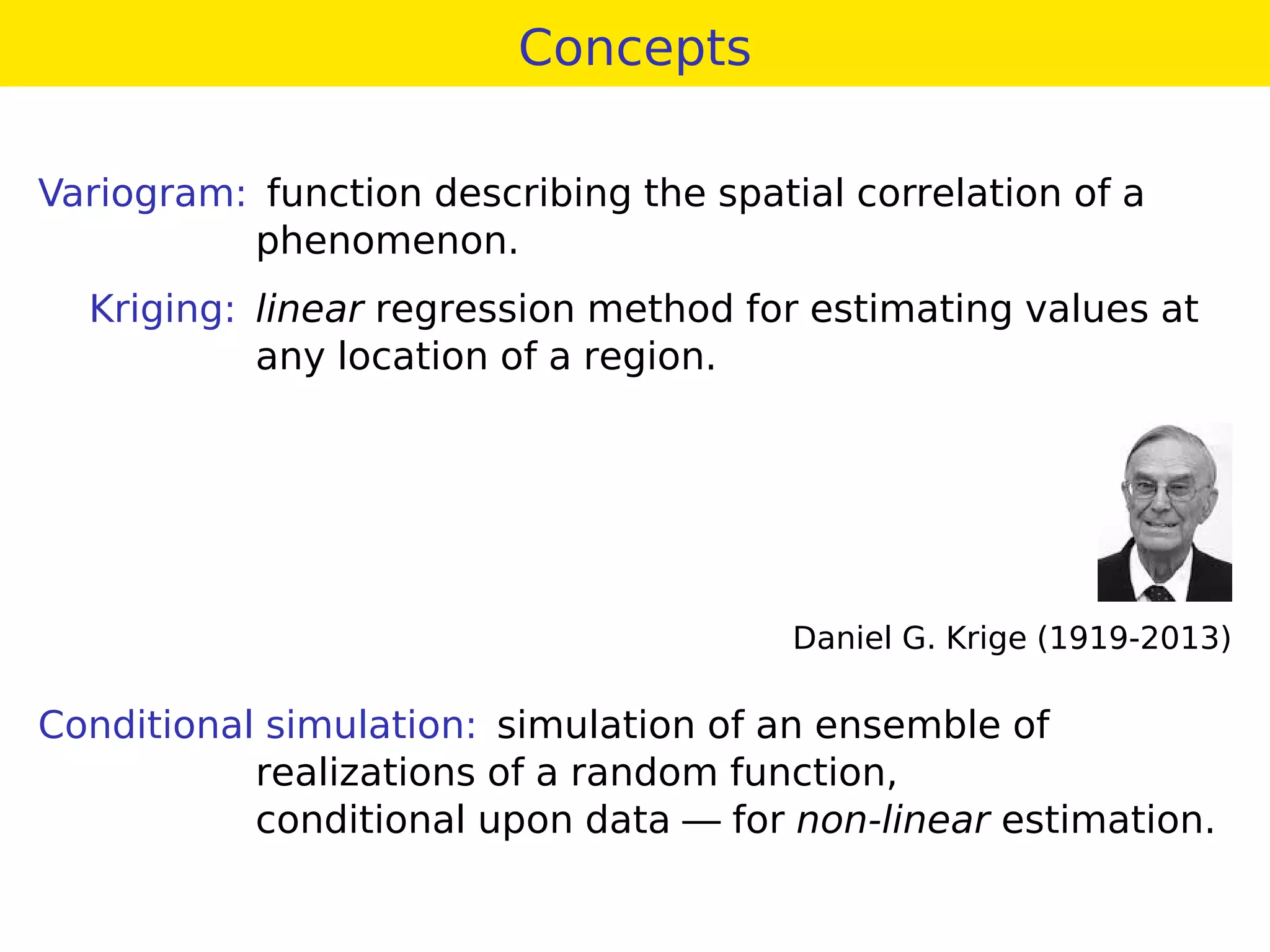
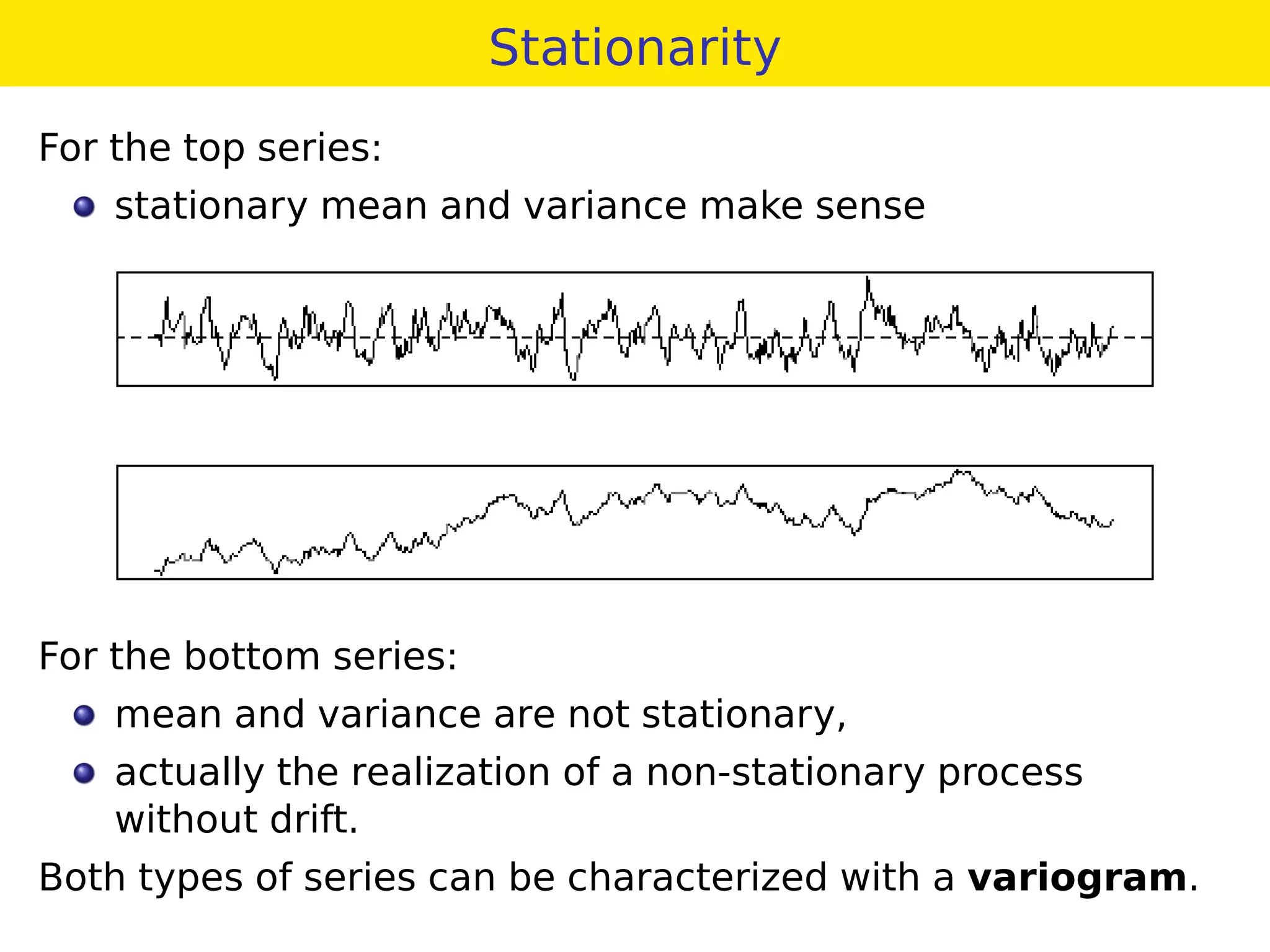
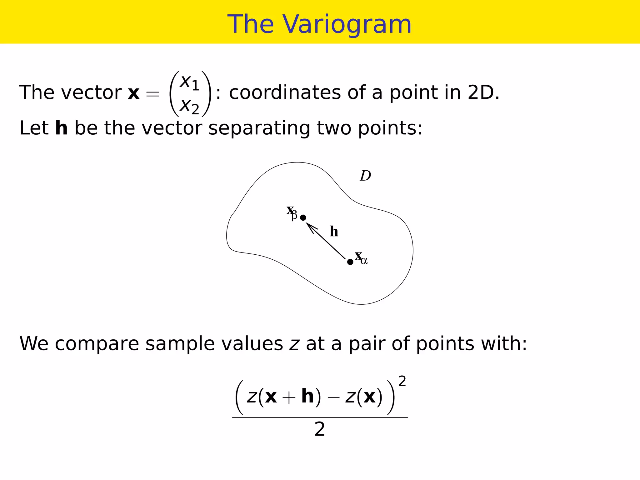
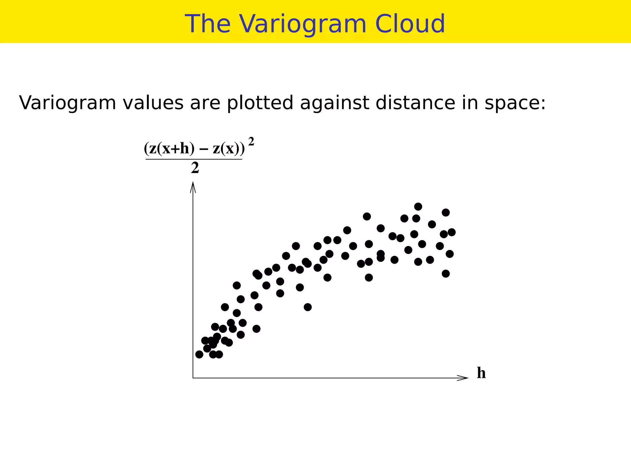
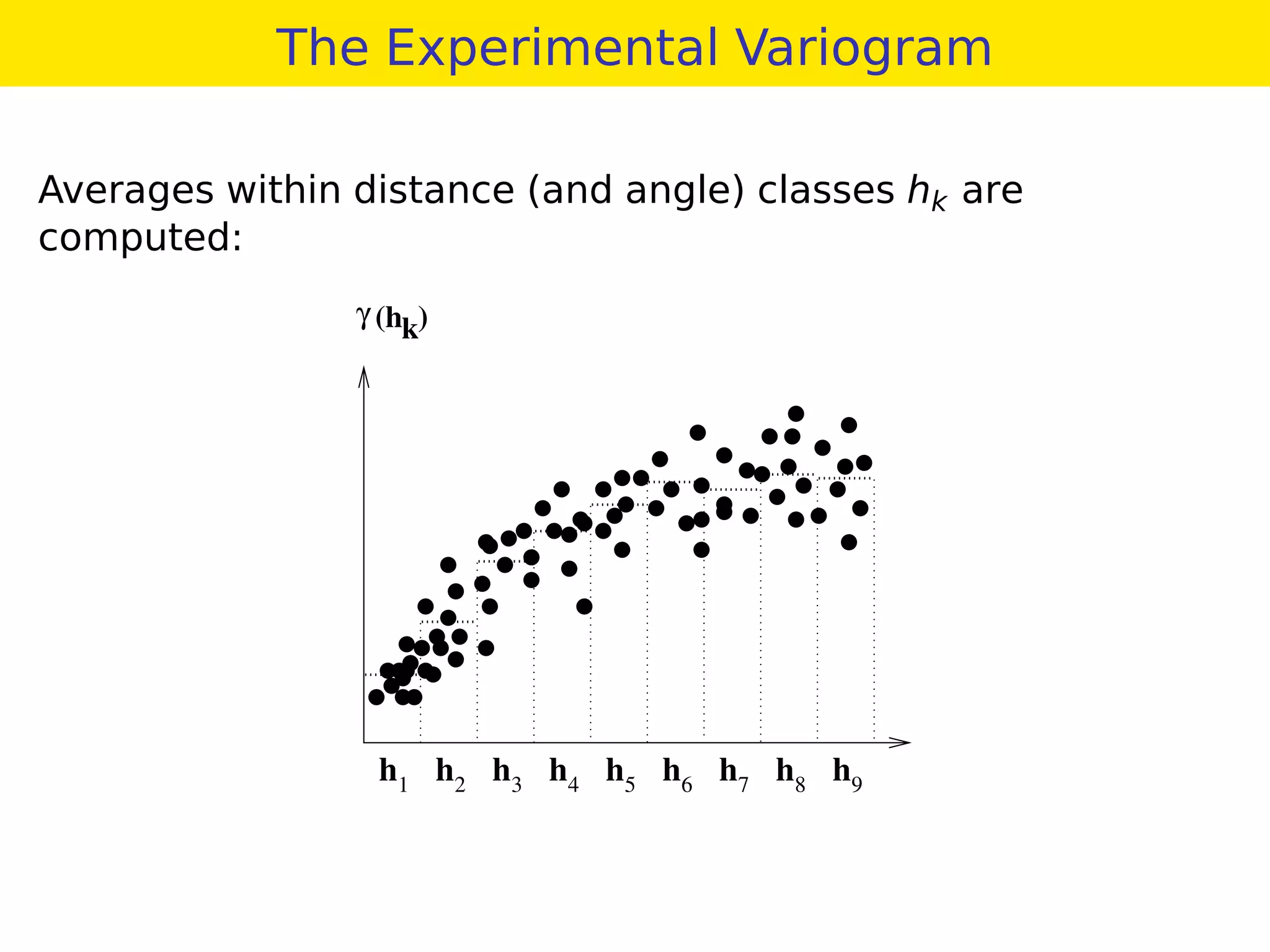
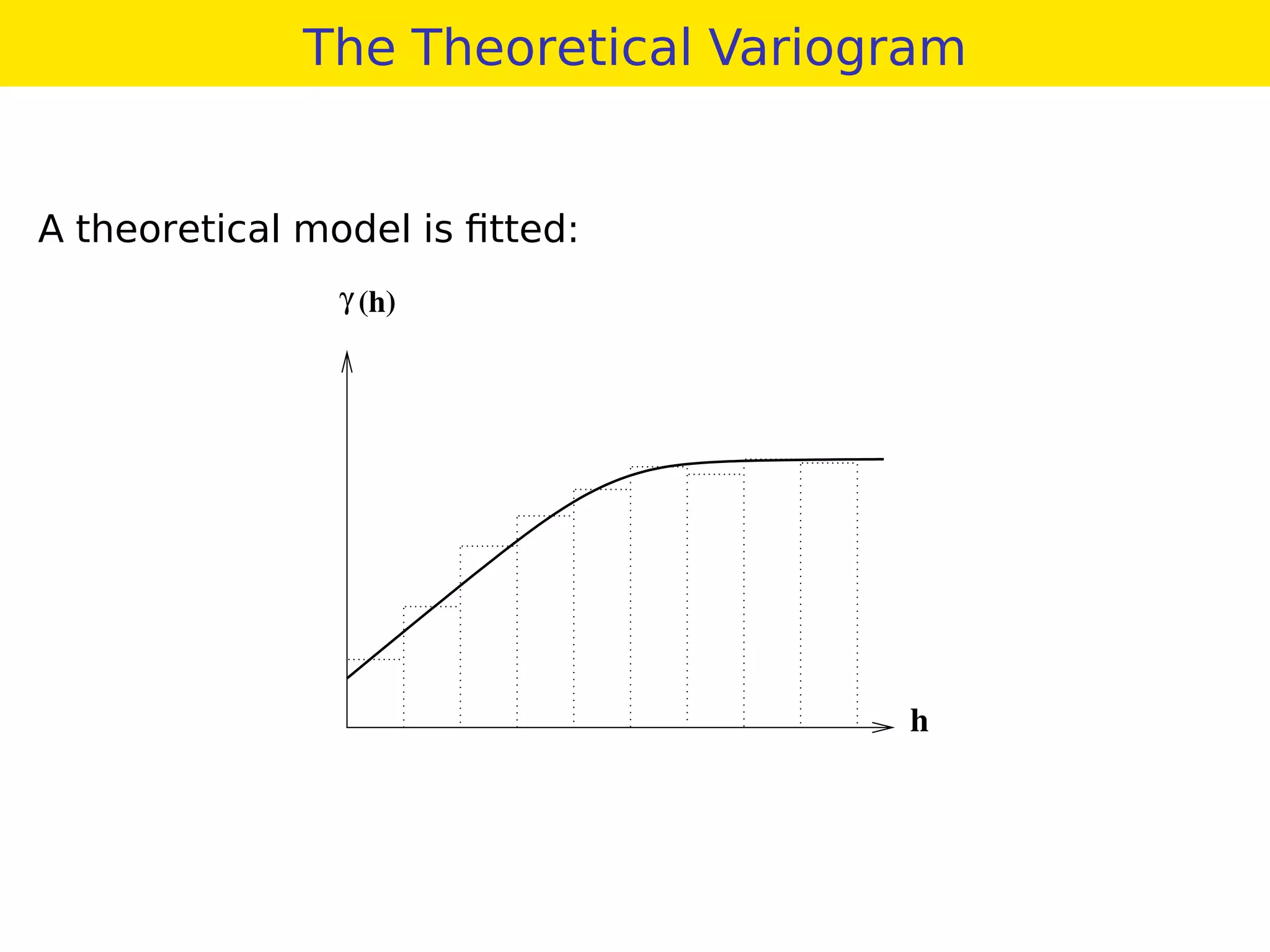
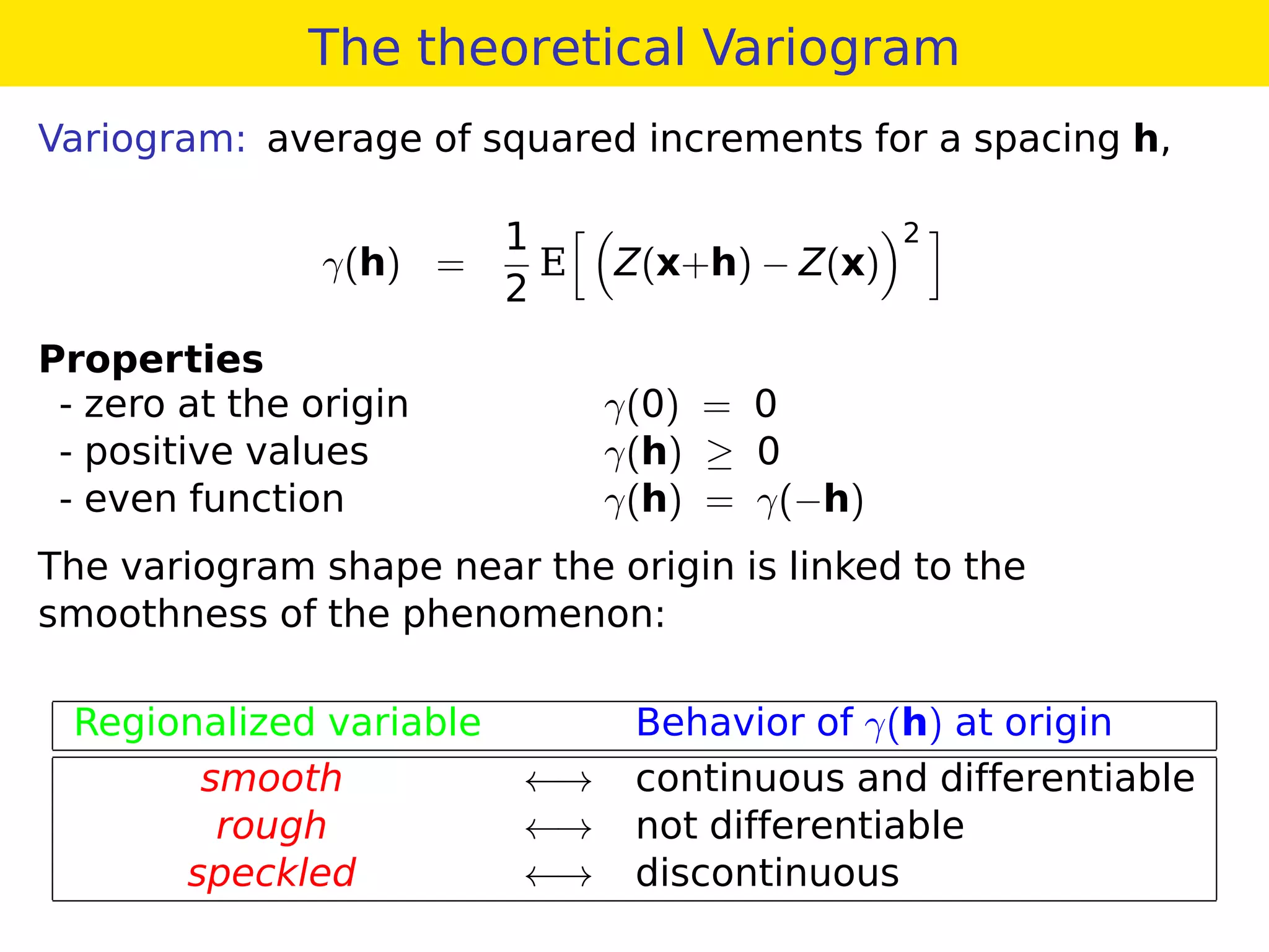
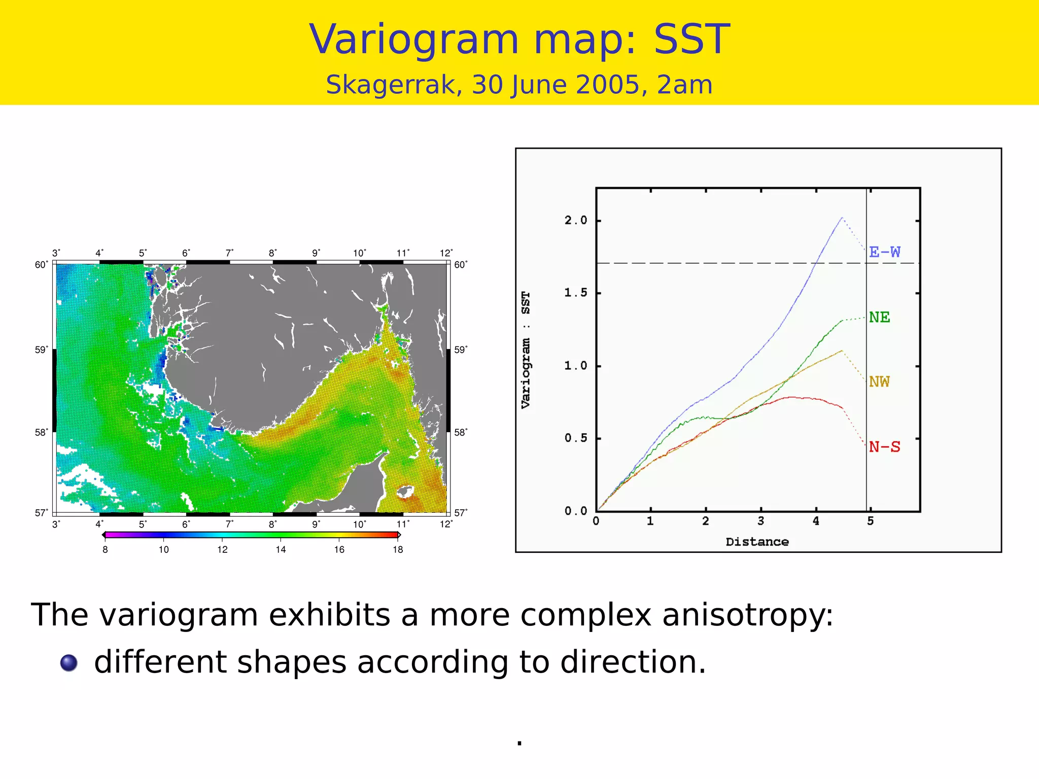
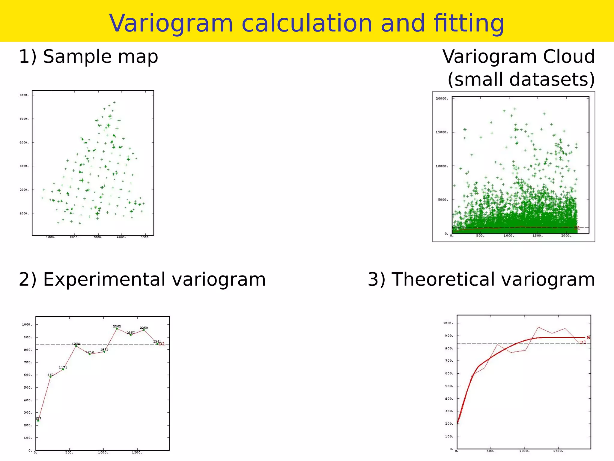
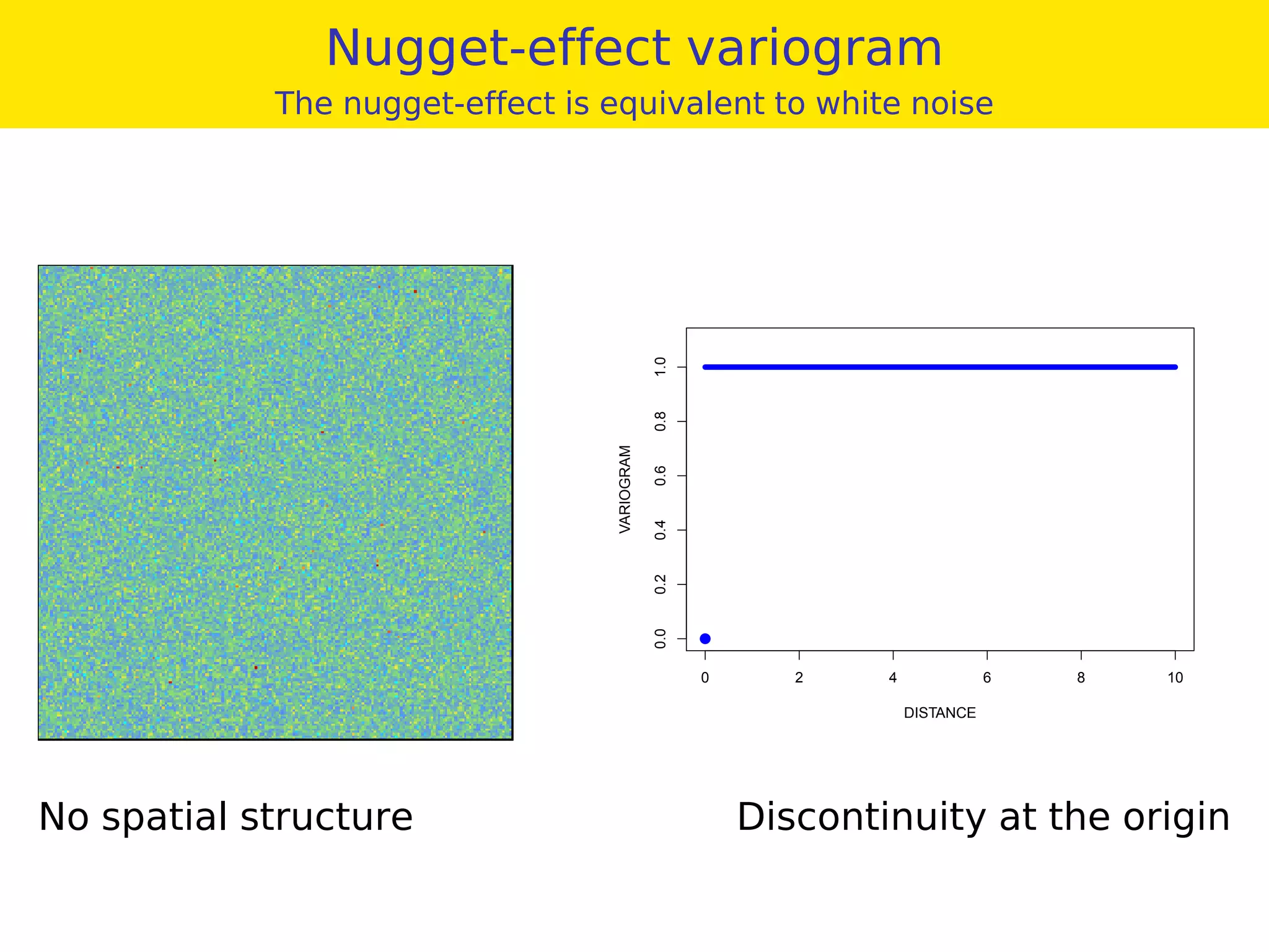
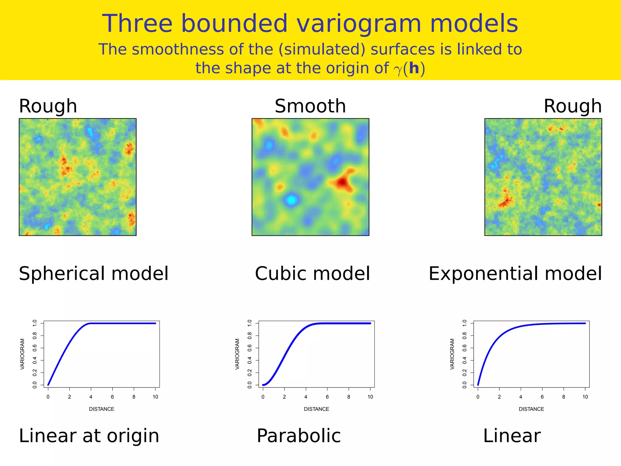
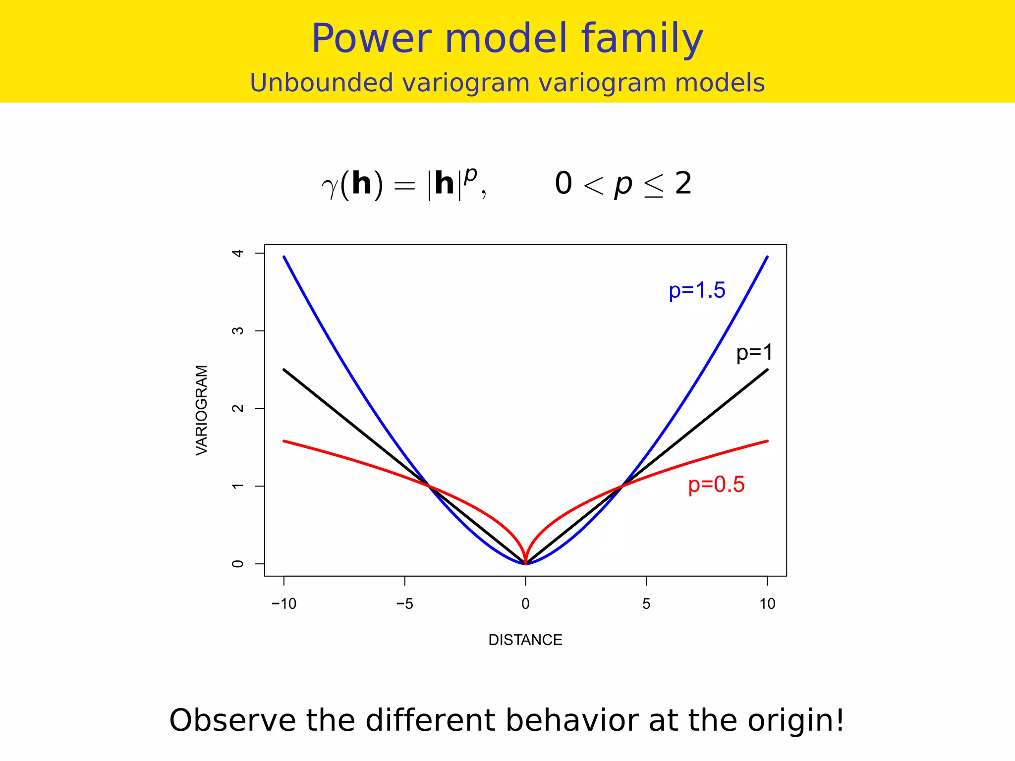
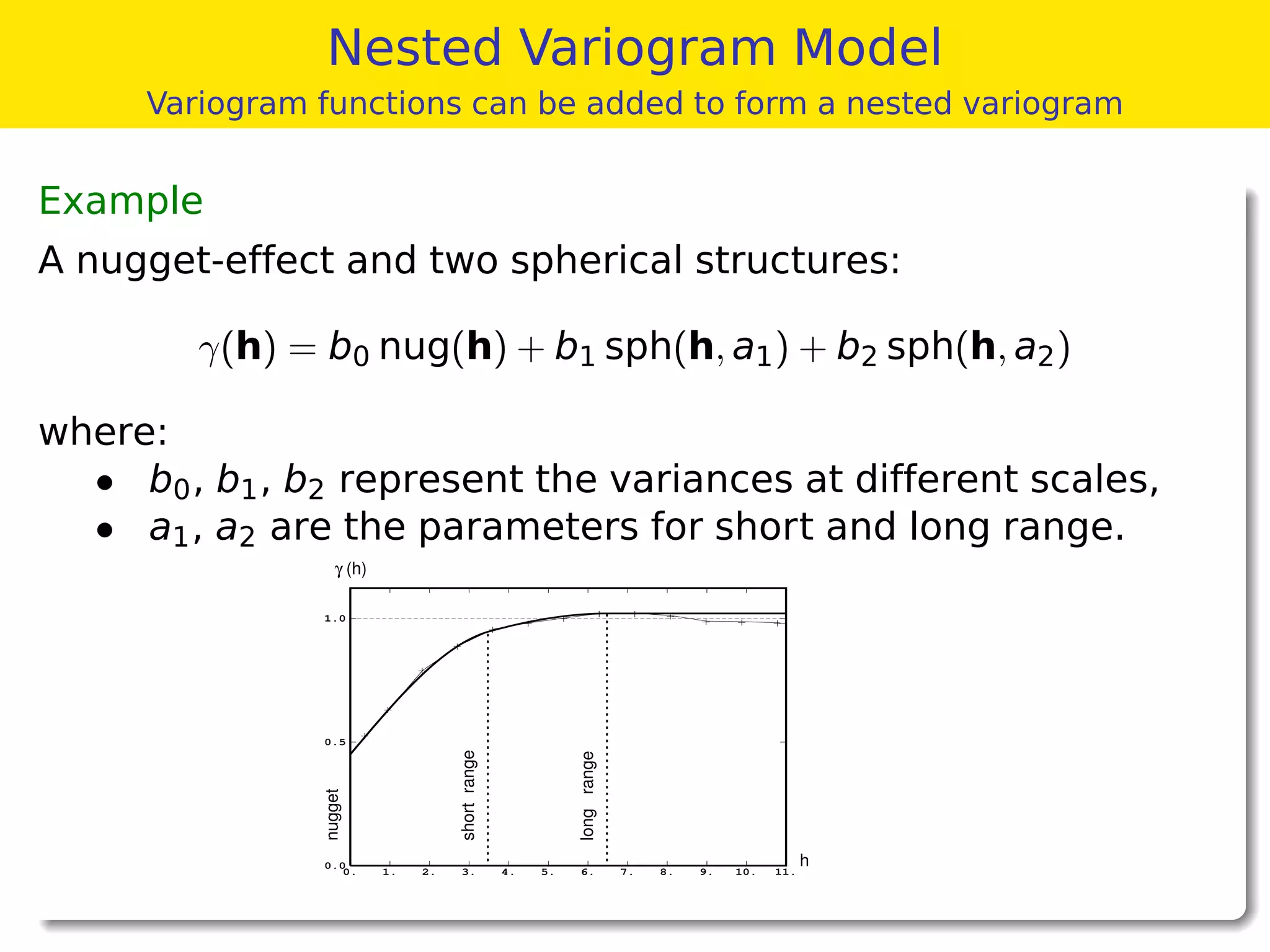
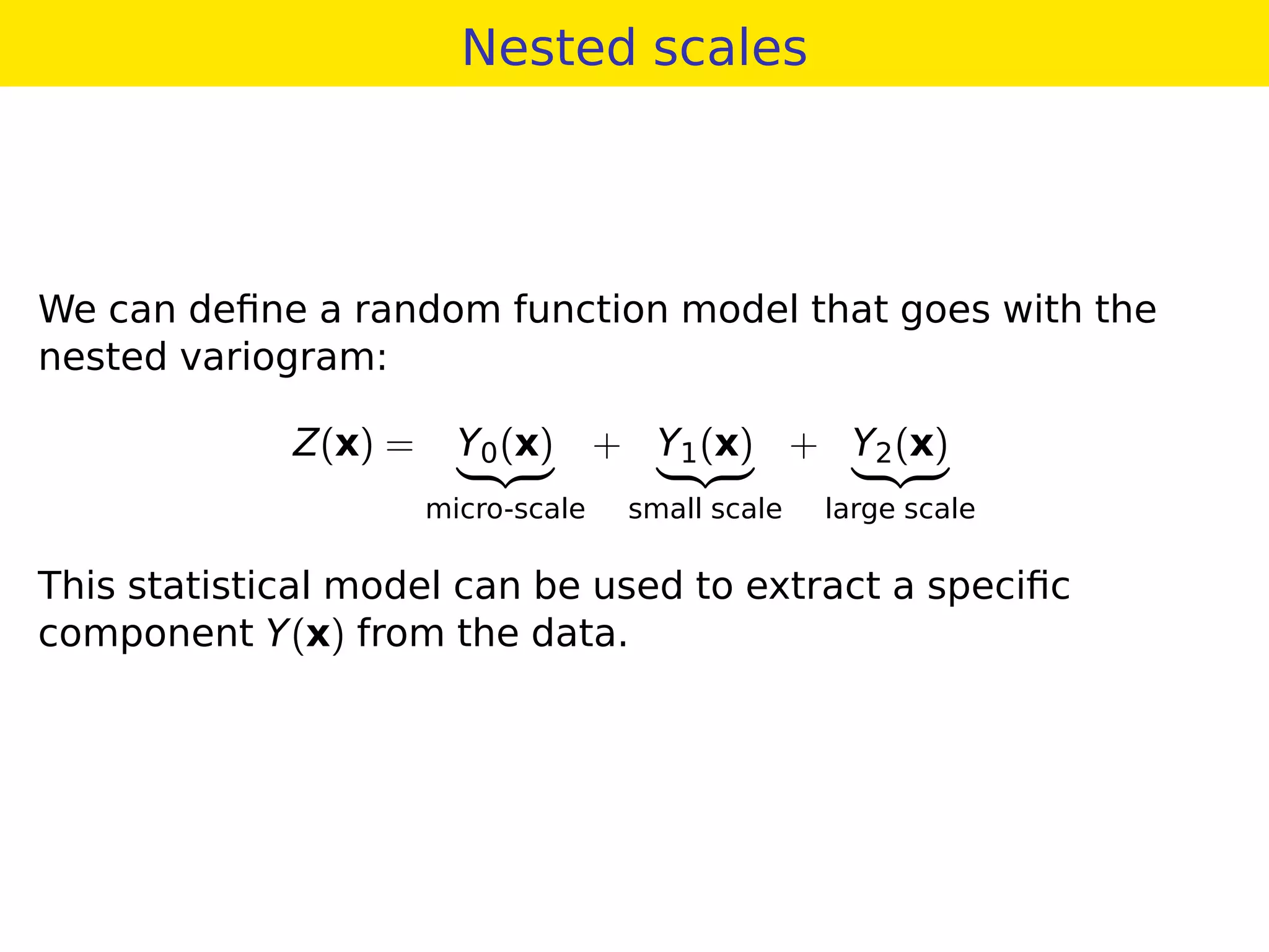
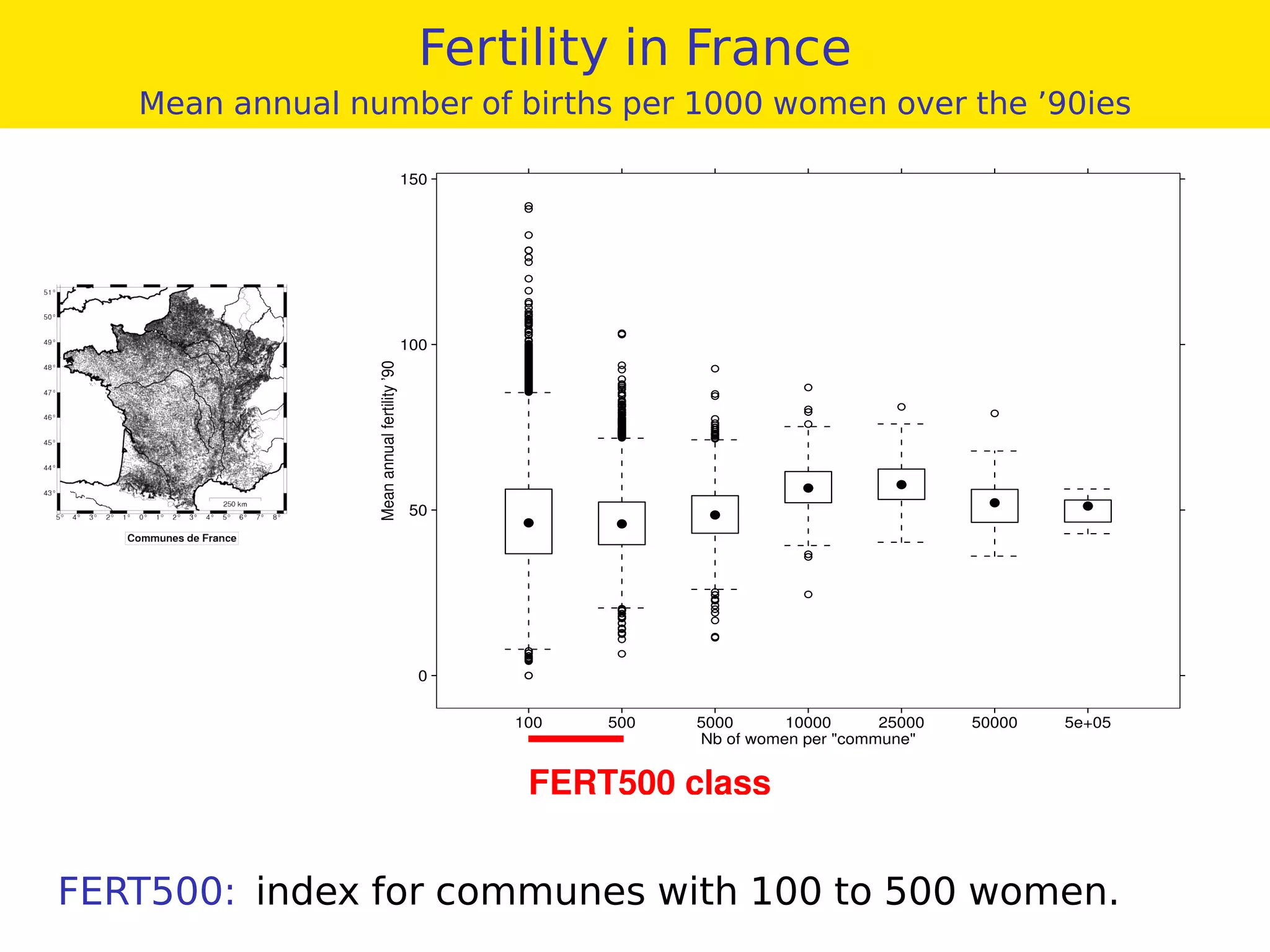
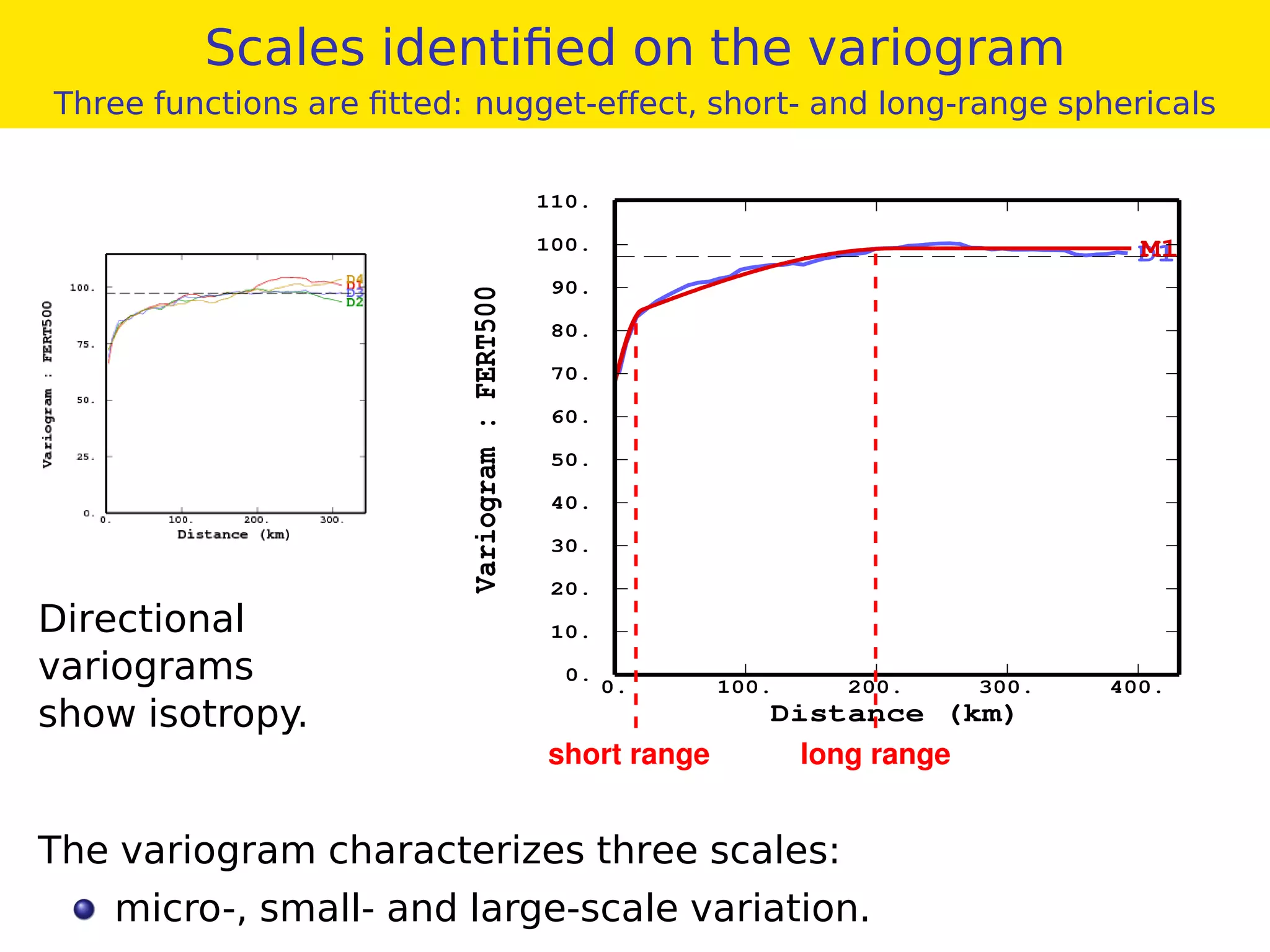
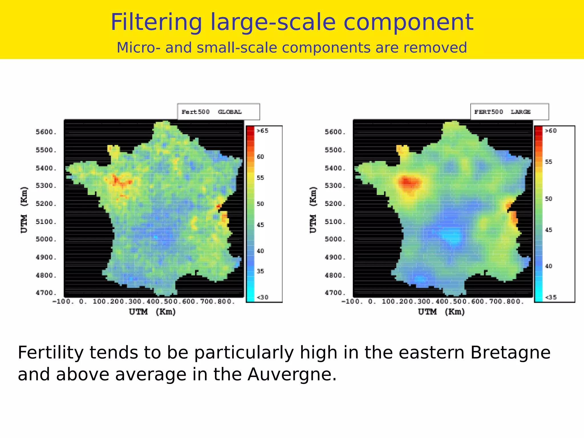
Basics in Geostatistics 1
Geostatistical structure analysis:
The variogram
Hans Wackernagel
MINES ParisTech
NERSC • April 2013
http://hans.wackernagel.free.fr
Basic concepts
Geostatistics
Hans Wackernagel (MINES ParisTech) Basics in Geostatistics 1 NERSC • April 2013 2 / 32
Geostatistics
Geostatistics is an application of
the theory of Regionalized Variables
to the problem of predicting spatial
phenomena.
Georges Matheron (1930-2000)
Note: the regionalized variable (reality) is viewed as a realization
of a random function, which is a collection of random variables.
Geostatistics has been applied to:
geology and mining since the ’50ies,
natural phenomena since the ’70ies.
It (re-)integrated mainstream statistics in the ’90ies.
Concepts
Variogram: function describing the spatial correlation of a
phenomenon.
Concepts
Variogram: function describing the spatial correlation of a
phenomenon.
Kriging: linear regression method for estimating values at
any location of a region.
Daniel G. Krige (1919-2013)
Concepts
Variogram: function describing the spatial correlation of a
phenomenon.
Kriging: linear regression method for estimating values at
any location of a region.
Daniel G. Krige (1919-2013)
Conditional simulation: simulation of an ensemble of
realizations of a random function,
conditional upon data — for non-linear estimation.
Stationarity
For the top series:
stationary mean and variance make sense
For the bottom series:
mean and variance are not stationary,
actually the realization of a non-stationary process
without drift.
Both types of series can be characterized with a variogram.
Structure analysis
Variogram
Hans Wackernagel (MINES ParisTech) Basics in Geostatistics 1 NERSC • April 2013 6 / 32
The Variogram
The vector x =
x1
x2
: coordinates of a point in 2D.
Let h be the vector separating two points:
G
G
h
D
x
x
β
α
We compare sample values z at a pair of points with:
z(x + h) − z(x)
2
2
The Variogram Cloud
Variogram values are plotted against distance in space:
GG
GG
GG
G
GG G
GGG
GG
G G G
G
G
G
G G
G
G G
GG
G
G
G
G
G
G G
G
G
G
G
G
G
G
G
G
G
G
G
GGG
G
G
G
G
G
G
G GG
GG
G
G
G
G
G
G G
G
G
G
G
G G
G
G
G
h
(z(x+h) − z(x))
2
2
The Experimental Variogram
Averages within distance (and angle) classes hk are
computed:
GG
GG
GG
G
GG G
GGG
GG
G G G
G
G
G
G G
G
G G
GG
G
G
G
G
G
G G
G
G
G
G
G
G
G
G
G
G
G
G
GGG
G
G
G
G
G
G
G GG
GG
G
G
G
G
G
G G
G
G
G
G
G G
G
G
G
h hh h h h h hh1 2 3 4 5 6 7 8 9
γ k(h )
The Theoretical Variogram
A theoretical model is fitted:
γ
h
(h)
The theoretical Variogram
Variogram: average of squared increments for a spacing h,
γ(h) =
1
2
E Z(x+h) − Z(x)
2
Properties
- zero at the origin γ(0) = 0
- positive values γ(h) ≥ 0
- even function γ(h) = γ(−h)
The variogram shape near the origin is linked to the
smoothness of the phenomenon:
Regionalized variable Behavior of γ(h) at origin
smooth ←→ continuous and differentiable
rough ←→ not differentiable
speckled ←→ discontinuous
Structure analysis
The empirical variogram
Hans Wackernagel (MINES ParisTech) Basics in Geostatistics 1 NERSC • April 2013 12 / 32
Empirical variogram
Variogram: average of squared increments for a class hk,
γ (hk) =
1
2 N(hk)
xα−xβ∈hk
(Z(xα) − Z(xβ))2
where N(hk) is the number of lags h = xα−xβ within
the distance (and angle) class hk.
Example 1D
Transect :
Example 1D
Transect :
γ (1) =
1
2 × 9
(02
+ 22
+ 02
+ 12
+ 32
+ 42
+ 22
+ 42
+ 02
) = 2.78
γ (2) =
1
2 × 8
(22
+ 22
+ 12
+ 22
+ 12
+ 62
+ 62
+ 42
) = 6.38
Example 1D
Transect :
γ (1) =
1
2 × 9
(02
+ 22
+ 02
+ 12
+ 32
+ 42
+ 22
+ 42
+ 02
) = 2.78
γ (2) =
1
2 × 8
(22
+ 22
+ 12
+ 22
+ 12
+ 62
+ 62
+ 42
) = 6.38
Example 2D
The directional variograms overlay: the variogram is isotropic.
Variogram: anisotropy
Computing the variogram for two pairs of directions.
The anisotropy becomes apparent when computing the pair of
directions 45 and 135 degrees.
Variogram map: SST
Skagerrak, 30 June 2005, 2am
The variogram exhibits a more complex anisotropy:
different shapes according to direction.
.
Structure analysis
Variogram model
Hans Wackernagel (MINES ParisTech) Basics in Geostatistics 1 NERSC • April 2013 18 / 32
Variogram calculation and fitting
1) Sample map Variogram Cloud
(small datasets)
2) Experimental variogram 3) Theoretical variogram
Nugget-effect variogram
The nugget-effect is equivalent to white noise
0 2 4 6 8 10
0.00.20.40.60.81.0
DISTANCE
VARIOGRAM
q
No spatial structure Discontinuity at the origin
Three bounded variogram models
The smoothness of the (simulated) surfaces is linked to
the shape at the origin of γ(h)
Rough Smooth Rough
Spherical model Cubic model Exponential model
0 2 4 6 8 10
0.00.20.40.60.81.0
DISTANCE
VARIOGRAM
0 2 4 6 8 10
0.00.20.40.60.81.0
DISTANCE
VARIOGRAM
0 2 4 6 8 10
0.00.20.40.60.81.0
DISTANCE
VARIOGRAM
Linear at origin Parabolic Linear
Power model family
Unbounded variogram variogram models
γ(h) = |h|p
, 0 < p ≤ 2
−10 −5 0 5 10
01234
DISTANCE
VARIOGRAM
p=1.5
p=1
p=0.5
Observe the different behavior at the origin!
Nested variogram
Nested variogram
and corresponding random function model
Hans Wackernagel (MINES ParisTech) Basics in Geostatistics 1 NERSC • April 2013 23 / 32
Nested Variogram Model
Variogram functions can be added to form a nested variogram
Example
A nugget-effect and two spherical structures:
γ(h) = b0 nug(h) + b1 sph(h, a1) + b2 sph(h, a2)
where:
• b0, b1, b2 represent the variances at different scales,
• a1, a2 are the parameters for short and long range.
0. 1. 2. 3. 4. 5. 6. 7. 8. 9. 10. 11.
0.0
0.5
1.0
nugget
longrange
shortrange
(h)γ
h
Nested scales
We can define a random function model that goes with the
nested variogram:
Z(x) = Y0(x)
micro-scale
+ Y1(x)
small scale
+ Y2(x)
large scale
This statistical model can be used to extract a specific
component Y(x) from the data.
Filtering
Case study: human fertility in France
Hans Wackernagel (MINES ParisTech) Basics in Geostatistics 1 NERSC • April 2013 26 / 32
Fertility in France
Mean annual number of births per 1000 women over the ’90ies
Nb of women per "commune"
Meanannualfertility’90
0
50
100
150
100 500 5000 10000 25000 50000 5e+05
FERT500 class
FERT500: index for communes with 100 to 500 women.
Scales identified on the variogram
Three functions are fitted: nugget-effect, short- and long-range sphericals
Directional
variograms
show isotropy.
D1M1
0. 100. 200. 300. 400.
Distance (km)
0.
10.
20.
30.
40.
50.
60.
70.
80.
90.
100.
110.
Variogram:FERT500
long rangeshort range
The variogram characterizes three scales:
micro-, small- and large-scale variation.
Filtering large-scale component
Micro- and small-scale components are removed
Fertility tends to be particularly high in the eastern Bretagne
and above average in the Auvergne.
Conclusion
Summary
We have seen that:
the variogram model characterizes the variability at
different scales,
a random function model with several components can be
associated to the structures identified on the variogram,
these components can be extracted by kriging and
mapped.
We will see next how to formulate different kriging algorithms.
Hans Wackernagel (MINES ParisTech) Basics in Geostatistics 1 NERSC • April 2013 30 / 32
References
JP Chilès and P Delfiner.
Geostatistics: Modeling Spatial Uncertainty.
Wiley, New York, 2nd edition, 2012.
P. Diggle, M. Fuentes, A.E. Gelfand, and P. Guttorp, editors.
Handbook of Spatial Statistics.
Chapman Hall, 2010.
C Lantuéjoul.
Geostatistical Simulation: Models and Algorithms.
Springer-Verlag, Berlin, 2002.
H Wackernagel.
Multivariate Geostatistics: an Introduction with
Applications.
Springer-Verlag, Berlin, 3rd edition, 2003.
Software
Public domain
The free (though not open source) geostatistical software
package RgeoS is available for use in R at:
http://rgeos.free.fr
R is free and available at http://www.r-project.org/
R can be used in a matlab-like graphical environement by
installing additionnally: http://www.rstudio.com/ide/
Commercial
The window and menu driven software Isatis is available
from: http://www.geovariances.com

Basics1variogram

  • 1.
    Basics in Geostatistics1 Geostatistical structure analysis: The variogram Hans Wackernagel MINES ParisTech NERSC • April 2013 http://hans.wackernagel.free.fr
  • 2.
    Basic concepts Geostatistics Hans Wackernagel(MINES ParisTech) Basics in Geostatistics 1 NERSC • April 2013 2 / 32
  • 3.
    Geostatistics Geostatistics is anapplication of the theory of Regionalized Variables to the problem of predicting spatial phenomena. Georges Matheron (1930-2000) Note: the regionalized variable (reality) is viewed as a realization of a random function, which is a collection of random variables. Geostatistics has been applied to: geology and mining since the ’50ies, natural phenomena since the ’70ies. It (re-)integrated mainstream statistics in the ’90ies.
  • 4.
    Geostatistics Geostatistics is anapplication of the theory of Regionalized Variables to the problem of predicting spatial phenomena. Georges Matheron (1930-2000) Note: the regionalized variable (reality) is viewed as a realization of a random function, which is a collection of random variables. Geostatistics has been applied to: geology and mining since the ’50ies, natural phenomena since the ’70ies. It (re-)integrated mainstream statistics in the ’90ies.
  • 5.
    Concepts Variogram: function describingthe spatial correlation of a phenomenon.
  • 6.
    Concepts Variogram: function describingthe spatial correlation of a phenomenon. Kriging: linear regression method for estimating values at any location of a region. Daniel G. Krige (1919-2013)
  • 7.
    Concepts Variogram: function describingthe spatial correlation of a phenomenon. Kriging: linear regression method for estimating values at any location of a region. Daniel G. Krige (1919-2013) Conditional simulation: simulation of an ensemble of realizations of a random function, conditional upon data — for non-linear estimation.
  • 8.
    Stationarity For the topseries: stationary mean and variance make sense For the bottom series: mean and variance are not stationary, actually the realization of a non-stationary process without drift. Both types of series can be characterized with a variogram.
  • 9.
    Structure analysis Variogram Hans Wackernagel(MINES ParisTech) Basics in Geostatistics 1 NERSC • April 2013 6 / 32
  • 10.
    The Variogram The vectorx = x1 x2 : coordinates of a point in 2D. Let h be the vector separating two points: G G h D x x β α We compare sample values z at a pair of points with: z(x + h) − z(x) 2 2
  • 11.
    The Variogram Cloud Variogramvalues are plotted against distance in space: GG GG GG G GG G GGG GG G G G G G G G G G G G GG G G G G G G G G G G G G G G G G G G G GGG G G G G G G G GG GG G G G G G G G G G G G G G G G G h (z(x+h) − z(x)) 2 2
  • 12.
    The Experimental Variogram Averageswithin distance (and angle) classes hk are computed: GG GG GG G GG G GGG GG G G G G G G G G G G G GG G G G G G G G G G G G G G G G G G G G GGG G G G G G G G GG GG G G G G G G G G G G G G G G G G h hh h h h h hh1 2 3 4 5 6 7 8 9 γ k(h )
  • 13.
    The Theoretical Variogram Atheoretical model is fitted: γ h (h)
  • 14.
    The theoretical Variogram Variogram:average of squared increments for a spacing h, γ(h) = 1 2 E Z(x+h) − Z(x) 2 Properties - zero at the origin γ(0) = 0 - positive values γ(h) ≥ 0 - even function γ(h) = γ(−h) The variogram shape near the origin is linked to the smoothness of the phenomenon: Regionalized variable Behavior of γ(h) at origin smooth ←→ continuous and differentiable rough ←→ not differentiable speckled ←→ discontinuous
  • 15.
    Structure analysis The empiricalvariogram Hans Wackernagel (MINES ParisTech) Basics in Geostatistics 1 NERSC • April 2013 12 / 32
  • 16.
    Empirical variogram Variogram: averageof squared increments for a class hk, γ (hk) = 1 2 N(hk) xα−xβ∈hk (Z(xα) − Z(xβ))2 where N(hk) is the number of lags h = xα−xβ within the distance (and angle) class hk.
  • 17.
  • 18.
    Example 1D Transect : γ(1) = 1 2 × 9 (02 + 22 + 02 + 12 + 32 + 42 + 22 + 42 + 02 ) = 2.78 γ (2) = 1 2 × 8 (22 + 22 + 12 + 22 + 12 + 62 + 62 + 42 ) = 6.38
  • 19.
    Example 1D Transect : γ(1) = 1 2 × 9 (02 + 22 + 02 + 12 + 32 + 42 + 22 + 42 + 02 ) = 2.78 γ (2) = 1 2 × 8 (22 + 22 + 12 + 22 + 12 + 62 + 62 + 42 ) = 6.38
  • 20.
    Example 2D The directionalvariograms overlay: the variogram is isotropic.
  • 21.
    Variogram: anisotropy Computing thevariogram for two pairs of directions. The anisotropy becomes apparent when computing the pair of directions 45 and 135 degrees.
  • 22.
    Variogram map: SST Skagerrak,30 June 2005, 2am The variogram exhibits a more complex anisotropy: different shapes according to direction. .
  • 23.
    Structure analysis Variogram model HansWackernagel (MINES ParisTech) Basics in Geostatistics 1 NERSC • April 2013 18 / 32
  • 24.
    Variogram calculation andfitting 1) Sample map Variogram Cloud (small datasets) 2) Experimental variogram 3) Theoretical variogram
  • 25.
    Nugget-effect variogram The nugget-effectis equivalent to white noise 0 2 4 6 8 10 0.00.20.40.60.81.0 DISTANCE VARIOGRAM q No spatial structure Discontinuity at the origin
  • 26.
    Three bounded variogrammodels The smoothness of the (simulated) surfaces is linked to the shape at the origin of γ(h) Rough Smooth Rough Spherical model Cubic model Exponential model 0 2 4 6 8 10 0.00.20.40.60.81.0 DISTANCE VARIOGRAM 0 2 4 6 8 10 0.00.20.40.60.81.0 DISTANCE VARIOGRAM 0 2 4 6 8 10 0.00.20.40.60.81.0 DISTANCE VARIOGRAM Linear at origin Parabolic Linear
  • 27.
    Power model family Unboundedvariogram variogram models γ(h) = |h|p , 0 < p ≤ 2 −10 −5 0 5 10 01234 DISTANCE VARIOGRAM p=1.5 p=1 p=0.5 Observe the different behavior at the origin!
  • 28.
    Nested variogram Nested variogram andcorresponding random function model Hans Wackernagel (MINES ParisTech) Basics in Geostatistics 1 NERSC • April 2013 23 / 32
  • 29.
    Nested Variogram Model Variogramfunctions can be added to form a nested variogram Example A nugget-effect and two spherical structures: γ(h) = b0 nug(h) + b1 sph(h, a1) + b2 sph(h, a2) where: • b0, b1, b2 represent the variances at different scales, • a1, a2 are the parameters for short and long range. 0. 1. 2. 3. 4. 5. 6. 7. 8. 9. 10. 11. 0.0 0.5 1.0 nugget longrange shortrange (h)γ h
  • 30.
    Nested scales We candefine a random function model that goes with the nested variogram: Z(x) = Y0(x) micro-scale + Y1(x) small scale + Y2(x) large scale This statistical model can be used to extract a specific component Y(x) from the data.
  • 31.
    Filtering Case study: humanfertility in France Hans Wackernagel (MINES ParisTech) Basics in Geostatistics 1 NERSC • April 2013 26 / 32
  • 32.
    Fertility in France Meanannual number of births per 1000 women over the ’90ies Nb of women per "commune" Meanannualfertility’90 0 50 100 150 100 500 5000 10000 25000 50000 5e+05 FERT500 class FERT500: index for communes with 100 to 500 women.
  • 33.
    Scales identified onthe variogram Three functions are fitted: nugget-effect, short- and long-range sphericals Directional variograms show isotropy. D1M1 0. 100. 200. 300. 400. Distance (km) 0. 10. 20. 30. 40. 50. 60. 70. 80. 90. 100. 110. Variogram:FERT500 long rangeshort range The variogram characterizes three scales: micro-, small- and large-scale variation.
  • 34.
    Filtering large-scale component Micro-and small-scale components are removed Fertility tends to be particularly high in the eastern Bretagne and above average in the Auvergne.
  • 35.
    Conclusion Summary We have seenthat: the variogram model characterizes the variability at different scales, a random function model with several components can be associated to the structures identified on the variogram, these components can be extracted by kriging and mapped. We will see next how to formulate different kriging algorithms. Hans Wackernagel (MINES ParisTech) Basics in Geostatistics 1 NERSC • April 2013 30 / 32
  • 36.
    References JP Chilès andP Delfiner. Geostatistics: Modeling Spatial Uncertainty. Wiley, New York, 2nd edition, 2012. P. Diggle, M. Fuentes, A.E. Gelfand, and P. Guttorp, editors. Handbook of Spatial Statistics. Chapman Hall, 2010. C Lantuéjoul. Geostatistical Simulation: Models and Algorithms. Springer-Verlag, Berlin, 2002. H Wackernagel. Multivariate Geostatistics: an Introduction with Applications. Springer-Verlag, Berlin, 3rd edition, 2003.
  • 37.
    Software Public domain The free(though not open source) geostatistical software package RgeoS is available for use in R at: http://rgeos.free.fr R is free and available at http://www.r-project.org/ R can be used in a matlab-like graphical environement by installing additionnally: http://www.rstudio.com/ide/ Commercial The window and menu driven software Isatis is available from: http://www.geovariances.com