Production decline analysis is a traditional means of identifying well production problems and predicting well performance and life based on real production data. It uses empirical decline models that have little fundamental justifications. These models include • Exponential decline (constant fractional decline) • Harmonic decline, and • Hyperbolic decline.

1. Chapter 8: Production Decline Analysis
8.1 Introduction
Production decline analysis is a traditional means of identifying well production
problems and predicting well performance and life based on real production data. It uses
empirical decline models that have little fundamental justifications. These models include
• Exponential decline (constant fractional decline)
• Harmonic decline, and
• Hyperbolic decline.
While the hyperbolic decline model is more general, the other two models are
degenerations of the hyperbolic decline model. These three models are related through
the following relative decline rate equation (Arps, 1945):
d
bq
dt
dq
q
−=
1
(8.1)
where b and d are empirical constants to be determined based on production data. When d
= 0, Eq (8.1) degenerates to an exponential decline model, and when d = 1, Eq (8.1)
yields a harmonic decline model. When 0 < d < 1, Eq (8.1) derives a hyperbolic decline
model. The decline models are applicable to both oil and gas wells.
8.2 Exponential Decline
The relative decline rate and production rate decline equations for the exponential decline
model can be derived from volumetric reservoir model. Cumulative production
expression is obtained by integrating the production rate decline equation.
8.2.1 Relative Decline Rate
Consider an oil well drilled in a volumetric oil reservoir. Suppose the well’s production
rate starts to decline when a critical (lowest permissible) bottom hole pressure is reached.
Under the pseudo-steady state flow condition, the production rate at a given decline time
t can be expressed as:
⎥
⎦
⎤
⎢
⎣
⎡
+⎟⎟
⎠
⎞
⎜⎜
⎝
⎛
−
=
s
r
r
B
ppkh
q
w
e
c
t wf
472.0
ln2.141
)(
0 μ
(8.2)
where tp = average reservoir pressure at decline time t,
c
wfp = the critical bottom hole pressure maintained during the production decline.
The cumulative oil production of the well after the production decline time t can be
expressed as:
8-1

2. dt
s
r
r
B
ppkh
N
t
w
e
o
c
t
p
wf
∫
⎥
⎦
⎤
⎢
⎣
⎡
+⎟⎟
⎠
⎞
⎜⎜
⎝
⎛
−
=
0 472.0
ln2.141
)(
μ
(8.3)
The cumulative oil production after the production decline upon decline time t can also
be evaluated based on the total reservoir compressibility:
( t
o
it
p pp
B
Nc
N −= 0 ) (8.4)
where = total reservoir compressibility,tc
iN = initial oil in place in the well drainage area,
0p = average reservoir pressure at decline time zero.
Substituting Eq (8.3) into Eq (8.4) yields:
( t
o
it
t
w
e
o
c
t
pp
B
Nc
dt
s
r
r
B
ppkh wf
−=
⎥
⎦
⎤
⎢
⎣
⎡
+⎟⎟
⎠
⎞
⎜⎜
⎝
⎛
−
∫ 0
0 472.0
ln2.141
)(
μ
) (8.5)
Taking derivative on both sides of this equation with respect to time t gives the
differential equation for reservoir pressure:
dt
pd
Nc
s
r
r
ppkh t
it
w
e
c
t wf
−=
⎥
⎦
⎤
⎢
⎣
⎡
+⎟⎟
⎠
⎞
⎜⎜
⎝
⎛
−
472.0
ln2.141
)(
μ
(8.6)
Since the left-hand-side of this equation is q and Eq (8.2) gives
dt
pd
s
r
r
B
kh
dt
dq t
w
e
⎥
⎦
⎤
⎢
⎣
⎡
+⎟⎟
⎠
⎞
⎜⎜
⎝
⎛
=
472.0
ln2.141 0μ
(8.7)
Eq (8.6) becomes
dt
dq
kh
s
r
r
Nc
q
w
e
it ⎥
⎦
⎤
⎢
⎣
⎡
+⎟⎟
⎠
⎞
⎜⎜
⎝
⎛
−
=
472.0
ln2.141 μ
(8.8)
8-2

3. or the relative decline rate equation of
b
dt
dq
q
−=
1
(8.9)
where
⎥
⎦
⎤
⎢
⎣
⎡
+⎟⎟
⎠
⎞
⎜⎜
⎝
⎛
=
s
r
r
Nc
kh
b
w
e
it
472.0
ln2.141 μ
. (8.10)
8.2.2 Production Rate Decline
Equation (8.6) can be expressed as:
dt
pd
ppb tc
t wf
=−− )( (8.11)
By separation of variables, Eq (8.11) can be integrated
∫∫ −
=−
t
wf
p
p
c
t
t
t
pp
pd
dtb
0
)(0
(8.12)
to yield an equation for reservoir pressure decline:
( ) btcc
t epppp wfwf
−
−+= 0 (8.13)
Substituting Eq (8.13) into Eq (8.2) gives well production rate decline equation:
bt
w
e
o
c
e
s
r
r
B
ppkh
q wf −
⎥
⎦
⎤
⎢
⎣
⎡
+⎟⎟
⎠
⎞
⎜⎜
⎝
⎛
−
=
472.0
ln2.141
)( 0
μ
(8.14)
or
btc
o
it
epp
B
Nbc
q wf
−
−= )( 0 (8.15)
which is the exponential decline model commonly used for production decline analysis of
solution-gas-drive reservoirs. In practice, the following form of Eq (8.15) is used:
bt
ieqq −
= (8.16)
where qi is the production rate at t = 0.
It can be shown that b
n
n
e
q
q
q
q
q
q −
−
====
12
3
1
2
...... . That is, the fractional decline is constant
8-3

4. for exponential decline. As an exercise, this is left to the reader to prove.
8.2.3 Cumulative Production
Integration of Eq (8.16) over time gives an expression for the cumulative oil production
since decline of
∫∫
−
==
t
bt
i
t
p dteqqdtN
00
(8.17)
i.e.,
( )bti
p e
b
q
N −
−= 1 . (8.18)
Since , Eq (8.18) becomesbt
ieqq −
=
( qq
b
N ip −=
1
). (8.19)
8.2.4 Determination of Decline Rate
The constant b is called the continuous decline rate. Its value can be determined from
production history data. If production rate and time data are available, the b-value can be
obtained based on the slope of the straight line on a semi-log plot. In fact, taking
logarithm of Eq (8.16) gives:
( ) ( ) btqq i −= lnln (8.20)
which implies that the data should form a straight line with a slope of -b on the log(q)
versus t plot, if exponential decline is the right model. Picking up any two points, (t1, q1)
and (t2, q2), on the straight line will allow analytical determination of b-value because
( ) ( ) 11 lnln btqq i −= (8.21)
and
( ) ( ) 22 lnln btqq i −= (8.22)
give
( ) ⎟⎟
⎠
⎞
⎜⎜
⎝
⎛
−
=
2
1
12
ln
1
q
q
tt
b . (8.23)
If production rate and cumulative production data are available, the b-value can be
obtained based on the slope of the straight line on an Np versus q plot. In fact, rearranging
Eq (8.19) yields:
8-4

5. pi bNqq −= (8.24)
Picking up any two points, (Np1, q1) and (Np2, q2), on the straight line will allow analytical
determination of b-value because
11 pi bNqq −= (8.25)
and
22 pi bNqq −= (8.26)
give
12
21
pp NN
qq
b
−
−
= . (8.27)
Depending on the unit of time t, the b can have different units such as month-1
and year-1
.
The following relation can be derived:
dma bbb 36512 == . (8.28)
where ba, bm, and bd are annual, monthly, and daily decline rates.
8.2.5 Effective Decline Rate
Because the exponential function is not easy to use in hand calculations, traditionally the
effective decline rate has been used. Since for small x-values based on
Taylor’s expansion, holds true for small values of b. The b is substituted by
, the effective decline rate, in field applications. Thus Eq (8.16) becomes
xe x
−≈−
1
be b
−≈−
1
'b
( t
i bqq '1−= ) (8.29)
Again, it can be shown that '1......
12
3
1
2
b
q
q
q
q
q
q
n
n
−====
−
.
Depending on the unit of time t, the can have different units such as month-1
and year-
1
. The following relation can be derived:
'b
( ) ( ) ( )36512
'1'1'1 dma bbb −=−=− . (8.30)
where a, , and b d are annual, monthly, and daily effective decline rates.'b 'b m '
8-5

6. Example Problem 8-1:
Given that a well has declined from 100 stb/day to 96 stb/day during a one-month period,
use the exponential decline model to perform the following tasts:
a) Predict the production rate after 11 more months
b) Calculate the amount of oil produced during the first year
c) Project the yearly production for the well for the next 5 years.
Solution:
a) Production rate after 11 more months:
( ) ⎟⎟
⎠
⎞
⎜⎜
⎝
⎛
−
=
m
m
mm
m
q
q
tt
b
1
0
01
ln
1
/month04082.0
96
100
ln
1
1
=⎟
⎠
⎞
⎜
⎝
⎛
⎟
⎠
⎞
⎜
⎝
⎛
=
Rate at end of one year
( )
stb/day27.61100 1204082.0
01 === −−
eeqq tb
mm
m
If the effective decline rate b’ is used,
/month04.0
100
96100
'
0
10
=
−
=
−
=
m
mm
m
q
qq
b .
From
( ) ( )
/year3875.0'
getsone
04.01'1'1
1212
=
−=−=−
y
my
b
bb
Rate at end of one year
( ) ( ) stb/day27.613875.01100'101 =−=−= ybqq
b) The amount of oil produced during the first year:
8-6

7. ( ) /year48986.01204082.0 ==yb
stb858,28365
48986.0
27.6110010
1, =⎟
⎠
⎞
⎜
⎝
⎛ −
=
−
=
y
p
b
qq
N
or
( )
( ) stb858,281
001342.0
100
day
1
001342.0
42.30
1
96
100
ln
365001342.0
1, =−=
=⎟
⎠
⎞
⎜
⎝
⎛
⎥
⎦
⎤
⎢
⎣
⎡
⎟
⎠
⎞
⎜
⎝
⎛
=
−
eN
b
p
d
c) Yearly production for the next 5 years:
( )
( ) stb681,171
001342.0
27.61 365001342.0
2, =−= −
eN p
( )
stb/day54.37100 )2(1204082.0
2 === −−
eeqq bt
i
( )
( ) stb834,101
001342.0
54.37 365001342.0
3, =−= −
eN p
( )
stb/day00.23100 )3(1204082.0
3 === −−
eeqq bt
i
( )
( ) stb639,61
001342.0
00.23 365001342.0
4, =−= −
eNp
( )
stb/day09.14100 )4(1204082.0
4 === −−
eeqq bt
i
( )
( ) stb061,41
001342.0
09.14 365001342.0
5, =−= −
eNp
In summary,
8-7

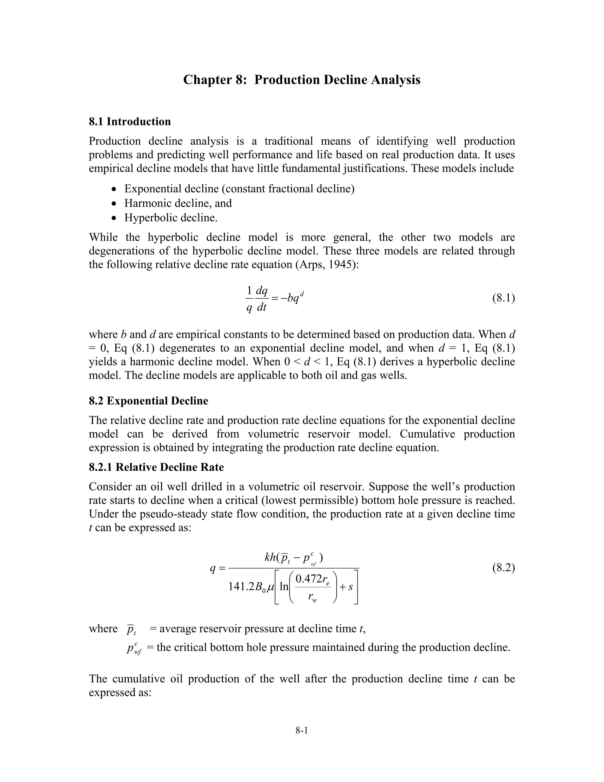
8. Year
Rate at End of Year
(stb/day)
Yearly Production
(stb)
0
1
2
3
4
5
100.00
61.27
37.54
23.00
14.09
8.64
-
28,858
17,681
10,834
6,639
4,061
68,073
8.3 Harmonic Decline
When d = 1, Eq (8.1) yields differential equation for a harmonic decline model:
bq
dt
dq
q
−=
1
(8.31)
which can be integrated as
bt
q
q
+
=
1
0
(8.32)
where q0 is the production rate at t = 0.
Expression for the cumulative production is obtained by integration:
∫=
t
p qdtN
0
which gives:
( bt
b
q
N p += 1ln0
). (8.33)
Combining Eqs (8.32) and (8.33) gives
( ) ( )[ qq
b
q
N p lnln 0
0
−= ]. (8.34)
8-8

9. 8.4 Hyperbolic Decline
When 0 < d < 1, integration of Eq (8.1) gives:
∫∫ −=+
tq
q
d
bdt
q
dq
0
1
0
(8.35)
which results in
( ) d
dbt
q
q /1
0
1+
= (8.36)
or
a
t
a
b
q
q
⎟
⎠
⎞
⎜
⎝
⎛
+
=
1
0
(8.37)
where a = 1/d.
Expression for the cumulative production is obtained by integration:
∫=
t
p qdtN
0
which gives:
( ) ⎥
⎥
⎦
⎤
⎢
⎢
⎣
⎡
⎟
⎠
⎞
⎜
⎝
⎛
+−
−
=
−a
p t
a
b
ab
aq
N
1
0
11
1
. (8.38)
Combining Eqs (8.37) and (8.38) gives
( ) ⎥
⎦
⎤
⎢
⎣
⎡
⎟
⎠
⎞
⎜
⎝
⎛
+−
−
= t
a
b
qq
ab
a
N p 1
1
0 . (8.39)
8.5 Model Identification
Production data can be plotted in different ways to identify a representative decline
model. If the plot of log(q) versus t shows a straight line (Figure 8-1), according to Eq
(8.20), the decline data follow an exponential decline model. If the plot of q versus Np
shows a straight line (Figure 8-2), according to Eq (8.24), an exponential decline model
should be adopted. If the plot of log(q) versus log(t) shows a straight line (Figure 8-3),
according to Eq (8.32), the decline data follow a harmonic decline model. If the plot of
Np versus log(q) shows a straight line (Figure 8-4), according to Eq (8.34), the harmonic
decline model should be used. If no straight line is seen in these plots, the hyperbolic
8-9

10. decline model may be verified by plotting the relative decline rate defined by Eq (8.1).
Figure 8-5 shows such a plot. This work can be easily performed with computer program
UcomS.exe.
q
t
Figure 8-1: A Semilog plot of q versus t indicating an exponential decline
q
pN
Figure 8-2: A plot of Np versus q indicating an exponential decline
8-10

11. q
t
Figure 8-3: A plot of log(q) versus log(t) indicating a harmonic decline
q
pN
Figure 8-4: A plot of Np versus log(q) indicating a harmonic decline
8-11

12. q
tq
q
Δ
Δ
−
Exponential Decline
Harmonic Decline
Hyperbolic Decline
Figure 8-5: A plot of relative decline rate versus production rate
8.6 Determination of Model Parameters
Once a decline model is identified, the model parameters a and b can be determined by
fitting the data to the selected model. For the exponential decline model, the b-value can
be estimated on the basis of the slope of the straight line in the plot of log(q) versus t (Eq
8.23). The b-value can also be determined based on the slope of the straight line in the
plot of q versus Np (Eq 8.27).
For the harmonic decline model, the b-value can be estimated on the basis of the slope of
the straight line in the plot of log(q) versus log(t) shows a straight line, or Eq (8.32):
1
1
0
1
t
q
q
b
−
= (8.40)
The b-value can also be estimated based on the slope of the straight line in the plot of Np
versus log(q) (Eq 8.34).
For the hyperbolic decline model, determination of a- and b-values is of a little tedious.
The procedure is shown in Figure 8-6.
8-12

13. 1. Select points (t1, q1)
and (t2, q2)
2. Read t3 at
3. Calculate
4. Find q0 at t = 0
5. Pick up any point (t*, q*)
6. Use
7. Finally
q
t
1
2
213 qqq =
21
2
3
321 2
ttt
ttt
a
b
−
−+
=⎟
⎠
⎞
⎜
⎝
⎛
a
t
a
b
q
q
⎟⎟
⎠
⎞
⎜⎜
⎝
⎛
⎟
⎠
⎞
⎜
⎝
⎛
+
=
*
0
*
1 ⎟⎟
⎠
⎞
⎜⎜
⎝
⎛
⎟
⎠
⎞
⎜
⎝
⎛
+
⎟⎟
⎠
⎞
⎜⎜
⎝
⎛
=
*
*
0
1log
log
t
a
b
q
q
a
a
a
b
b ⎟
⎠
⎞
⎜
⎝
⎛
=
q3
t3
(t*, q*)
Figure 8-6: Procedure for determining a- and b-values
Computer program UcomS.exe can be used for both model identification and model
parameter determination, as well as production rate prediction.
8.7 Illustrative Examples
Example Problem 8-2:
For the data given in Table 8-1, identify a suitable decline model, determine model
parameters, and project production rate until a marginal rate of 25 stb/day is reached.
Table 8-1: Production Data for Example Problem 8-2
t (Month) q (STB/D) t (Month) q (STB/D)
301.1912.00
332.8711.00
367.8810.00
406.579.00
449.338.00
496.597.00
548.816.00
606.535.00
670.324.00
740.823.00
818.732.00
904.841.00
301.1912.00
332.8711.00
367.8810.00
406.579.00
449.338.00
496.597.00
548.816.00
606.535.00
670.324.00
740.823.00
818.732.00
904.841.00
90.7224.00
100.2623.00
110.8022.00
122.4621.00
135.3420.00
149.5719.00
165.3018.00
182.6817.00
201.9016.00
223.1315.00
246.6014.00
272.5313.00
90.7224.00
100.2623.00
110.8022.00
122.4621.00
135.3420.00
149.5719.00
165.3018.00
182.6817.00
201.9016.00
223.1315.00
246.6014.00
272.5313.00
8-13

14. Solution:
A plot of log(q) versus t is presented in Figure 8-7 which shows a straight line.
According to Eq (8.20), the exponential decline model is applicable. This is further
evidenced by the relative decline rate shown in Figure 8-8.
Select points on the trend line:
t1= 5 months, q1 = 607 STB/D
t2= 20 months, q2 = 135 STB/D
Decline rate is calculated with Eq (8.23):
( )
1/month1.0
607
135
ln
205
1
=⎟
⎠
⎞
⎜
⎝
⎛
−
=b
Projected production rate profile is shown in Figure 8-9.
1
10
100
1000
10000
0 5 10 15 20 25 30
t (month)
q(STB/D)
8-14

15. Figure 8-7: A plot of log(q) versus t showing an exponential decline
0.05
0.06
0.07
0.08
0.09
0.1
0.11
0.12
0.13
0.14
0.15
3 203 403 603 803 1003
q (STB/D)
-Δq/Δt/q(Month-1
)
Figure 8-8: Relative decline rate plot showing exponential decline
0
100
200
300
400
500
600
700
800
900
1000
0 10 20 30
t (month)
q(STB/D
40
)
Figure 8-9: Projected production rate by an exponential decline model
Example Problem 8-3:
For the data given in Table 8-2, identify a suitable decline model, determine model
parameters, and project production rate till the end of the 5th
year.
8-15

16. Table 8-2: Production Data for Example Problem 8-3
t (year) q (1000 STB/D) t (year) q (1000 STB/D)
5.682.00
5.811.90
5.941.80
6.081.70
6.221.60
6.371.50
6.531.40
6.691.30
6.871.20
7.051.10
7.251.00
7.450.90
7.670.80
7.900.70
8.140.60
8.400.50
8.680.40
8.980.30
9.290.20
5.682.00
5.811.90
5.941.80
6.081.70
6.221.60
6.371.50
6.531.40
6.691.30
6.871.20
7.051.10
7.251.00
7.450.90
7.670.80
7.900.70
8.140.60
8.400.50
8.680.40
8.980.30
9.290.20
4.033.90
4.093.80
4.163.70
4.223.60
4.293.50
4.363.40
4.443.30
4.513.20
4.593.10
4.673.00
4.762.90
4.842.80
4.942.70
5.032.60
5.132.50
5.232.40
5.342.30
5.452.20
5.562.10
4.033.90
4.093.80
4.163.70
4.223.60
4.293.50
4.363.40
4.443.30
4.513.20
4.593.10
4.673.00
4.762.90
4.842.80
4.942.70
5.032.60
5.132.50
5.232.40
5.342.30
5.452.20
5.562.10
Solution:
A plot of relative decline rate is shown in Figure 8-10 which clearly indicates a
harmonic decline model.
On the trend line, select
q0 = 10,000 stb/day at t = 0
q1 = 5,680 stb/day at t = 2 years
Therefore, Eq (8.40) gives:
1/year38.0
2
1
680,5
000,10
=
−
=b .
Projected production rate profile is shown in Figure 8-11.
8-16

17. 0.1
0.15
0.2
0.25
0.3
0.35
0.4
3.00 4.00 5.00 6.00 7.00 8.00 9.00 10.00
q (1000 STB/D)
-Δq/Δt/q(year-1
)
Figure 8-10: Relative decline rate plot showing harmonic declineplot showing harmonic decline
0
2
4
6
8
10
12
0.0 1.0 2.0 3.0 4.0 5.0 6.0
t (year)
q(1000STB/D)
Projected production rate by a harmonic decline modelProjected production rate by a harmonic decline modelFigure 8-11:Figure 8-11:
Example Problem 8-4:Example Problem 8-4:
For the data given in Table 8-3, identify a suitable decline model, determine model
rate till the end of the 5th
year.
Sol
ecline rate is shown in Figure 8-12 which clearly indicates a
line model.
Select poin
parameters, and project production
ution:
A plot of relative d
hyperbolic dec
ts:
8-17

18. t1 = 0.2 year , q1 = 9,280 stb/day
t2 = 3.8 years, q2 = 3,490 stb/day
Read from decline curve (Figure 8-13) t3 = 1.75 yaers at q3 = 5,670 stb/day.
Read from decline curve (Figure 8-13) q0 = 10,000 stb/day at t0 = 0.
Pick up point ( = 6,280 stb/day).
Projected production rate profile is shown in Figure 8-14.
Table 8-3: Production Dat for Example Problem 8-4
stb/day5,670)490,3)(280,9(3 ==q
217.0
)75.1(28.32.0
2
=
−+
=⎟
⎞
⎜
⎛ b
)8.3)(2.0()75.1( −⎠⎝ a
t*
= 1.4 yesrs, q*
a
5.322.00 5.322.00 3.344.00 3.344.00
5.461.90
5.611.80
5.771.70
5.931.60
6.101.50
6.281.40
6.471.30
6.671.20
6.871.10
7.091.00
7.320.90
7.550.80
7.810.70
8.070.60
8.350.50
8.640.40
8.950.30
9.280.20
9.630.10
5.461.90
5.611.80
5.771.70
5.931.60
6.101.50
6.281.40
6.471.30
6.671.20
6.871.10
7.091.00
7.320.90
7.550.80
7.810.70
8.070.60
8.350.50
8.640.40
8.950.30
9.280.20
9.630.10
3.413.90
3.493.80
3.563.70
3.643.60
3.713.50
3.803.40
3.883.30
3.973.20
4.063.10
4.153.00
4.252.90
4.352.80
4.462.70
4.572.60
4.682.50
4.802.40
4.922.30
5.052.20
5.182.10
3.413.90
3.493.80
3.563.70
3.643.60
3.713.50
3.803.40
3.883.30
3.973.20
4.063.10
4.153.00
4.252.90
4.352.80
4.462.70
4.572.60
4.682.50
4.802.40
4.922.30
5.052.20
5.182.10
t(year) q(1000STB/D) t(year) q(1000STB/D)
( )( )
75.1
)4.1(217.01log
280,6
=
+
⎠⎝=a
000,10
log ⎟
⎞
⎜
⎛
( ) 38.0)758.1(217.0 ==b
8-18

19. 0.2
0.22
0.24
0.26
0.28
0.3
0.32
0.34
0.36
0.38
3.00 4.00 5.00 6.00 7.00 8.00 9.00 10.00
-Δq/Δt/q(year-1
)
q (1000 STB/D)
Figure 8-12: Relative decline rate rbolic decline
Figure 8-13: Relative decline rate plot showing hyperbolic decline
plot showing hype
0
2
4
6
8
10
12
0.0 1.0 2.0 3.0 4.0 5.0
q(1000STB/D)
t (year)
8-19

20. 0
2
4
6
8
10
12
0.0 1.0 2.0 3.0 4.0 5.0 6.0
t (year)
q(1000STB/D)
Figure 8-14: Projected production rate by a hyperbolic decline model
* * * * *
Summary
This chapter presented empirical models and procedure of using the models to perform
production decline data analyses. Computer program UcomS.exe can be used for model
identification, model parameter determination, and production rate prediction.
References
Arps, J.J.: “ Analysis of Decline Curves,” Trans. AIME, 160, 228-247, 1945.
Golan, M. and Whitson, C.M.: Well Performance, International Human Resource
Development Corp., 122-125, 1986.
Economides, M.J., Hill, A.D., and Ehlig-Economides, C.: Petroleum Production
Systems, Prentice Hall PTR, Upper Saddle River, 516-519, 1994.
Problems
8.1 For the data given in the following table, identify a suitable decline model, determine
model parameters, and project production rate till the end of the 10th
year. Predict
yearly oil productions:
8-20

21. Time (year) Production Rate (1,000 stb/day)
0.1 9.63
0.2 9.29
0.3 8.98
0.4 8.68
0.5 8.4
0.6 8.14
0.7 7.9
0.8 7.67
0.9 7.45
1 7.25
1.1 7.05
1.2 6.87
1.3 6.69
1.4 6.53
1.5 6.37
1.6 6.22
1.7 6.08
1.8 5.94
1.9 5.81
2 5.68
2.1 5.56
2.2 5.45
2.3 5.34
2.4 5.23
2.5 5.13
2.6 5.03
2.7 4.94
2.8 4.84
2.9 4.76
3 4.67
3.1 4.59
3.2 4.51
3.3 4.44
3.4 4.36
8.2 For the data given in the following table, identify a suitable decline model, determine
model parameters, predict the time when the production rate will decline to a
marginal value of 500 stb/day, and the reverses to be recovered before the marginal
production rate is reached:
8-21

22. Time (year) Production Rate (stb/day)
0.1 9.63
0.2 9.28
0.3 8.95
0.4 8.64
0.5 8.35
0.6 8.07
0.7 7.81
0.8 7.55
0.9 7.32
1 7.09
1.1 6.87
1.2 6.67
1.3 6.47
1.4 6.28
1.5 6.1
1.6 5.93
1.7 5.77
1.8 5.61
1.9 5.46
2 5.32
2.1 5.18
2.2 5.05
2.3 4.92
2.4 4.8
2.5 4.68
2.6 4.57
2.7 4.46
2.8 4.35
2.9 4.25
3 4.15
3.1 4.06
3.2 3.97
3.3 3.88
3.4 3.8
8.3 For the data given in the following table, identify a suitable decline model, determine
model parameters, predict the time when the production rate will decline to a
marginal value of 50 Mscf/day, and the reverses to be recovered before the marginal
production rate is reached:
8-22

23. Time
(Month)
Production Rate
(Mscf/day)
1 904.84
2 818.73
3 740.82
4 670.32
5 606.53
6 548.81
7 496.59
8 449.33
9 406.57
10 367.88
11 332.87
12 301.19
13 272.53
14 246.6
15 223.13
16 201.9
17 182.68
18 165.3
19 149.57
20 135.34
21 122.46
22 110.8
23 100.26
24 90.72
8.4 For the data given in the following table, identify a suitable decline model, determine
model parameters, predict the time when the production rate will decline to a
marginal value of 50 stb/day, and yearly oil productions:
Time
(Month)
Production Rate
(stb/day)
1 1810
2 1637
3 1482
4 1341
5 1213
6 1098
7 993
8-23

24. 8-24
8 899
9 813
10 736
11 666
12 602
13 545
14 493
15 446
16 404
17 365
18 331
19 299
20 271
21 245
22 222
23 201
24 181