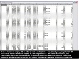
Downloaded 1,612 times


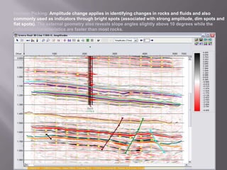
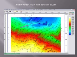
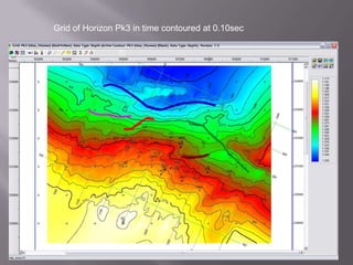
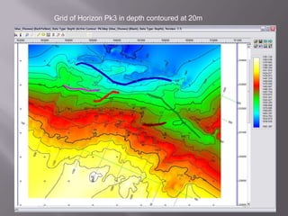
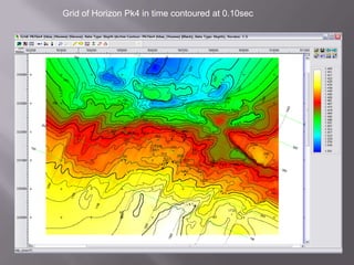
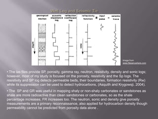
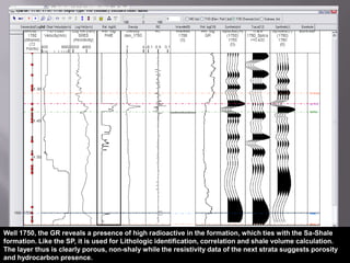
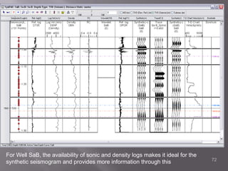
![An impedance log and reflection coefficient is generated from the velocity and density profiles. Where there is no density log, conversion is done with the resistivity log. The reflection coefficients are convolved with a seismic wavelet to produce a synthetic seismic trace. The seismic wavelet is obtained using a wavelet extraction from seismic data in each well study; the synthetic seismogram is then compared with the actual seismic trace from 200m around the well and aligned to match the reflection coefficient and GR or SP logs with a perfect correlation to be 1.Using Faust’s resistivity to velocity technique, I was able to generate density data by also converting the velocity to density logs. Some of the old logs were strictly for the reservoir and gave little insight and resolution to the upper strata. Lithology is derived and confirmed from the literature both from the seismogram interpretation and cross-plots of SP and porosity and density and sonic logs below:For well 903 which had resistivity logs without the needed porosity logs conversion was made to velocity log using Faust’s conversion from resistivity to velocity is: Velocity = C1 * Depth ^C2 * Resistivity^C3where C1 = 2374 (for Metric Z units), C2 = 0.1667, and C3 = 0.1667and from velocity to density using the formula Density = 108.2812*[Velocity (l)*4.0] where (l) = each log sample](https://image.slidesharecdn.com/gisapplicationspresentation-100309021038-phpapp01/85/Gis-Applications-Presentation-74-320.jpg)
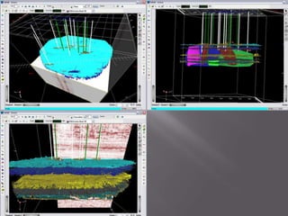


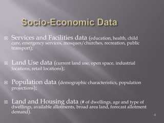
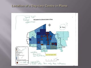
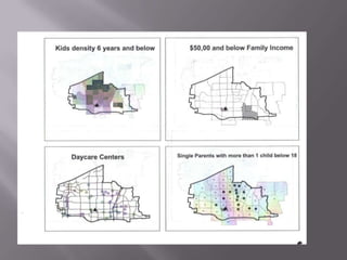
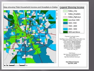
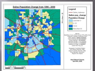
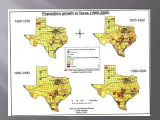
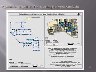
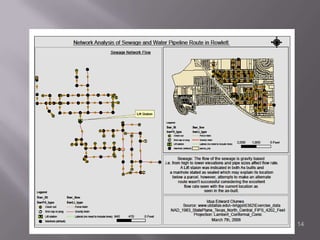
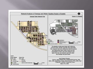
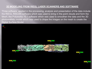
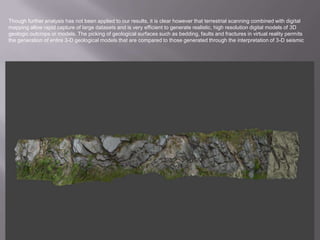
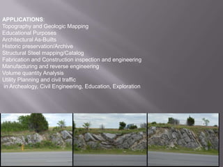
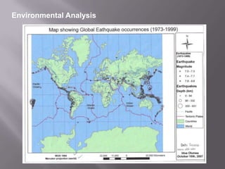
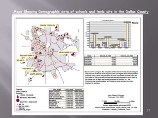
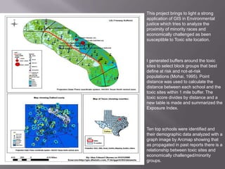
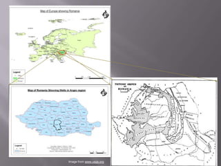
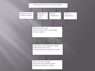
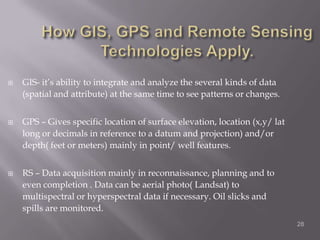
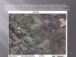
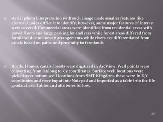
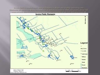
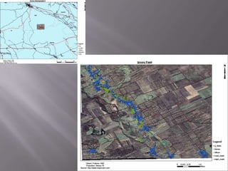
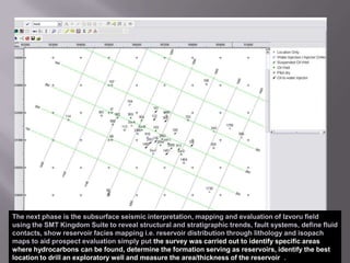
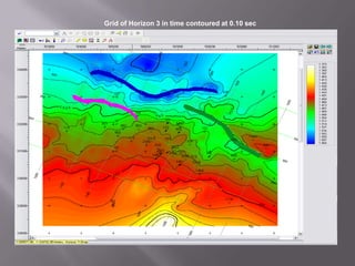
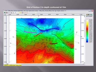
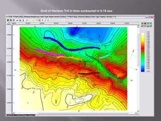
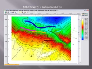
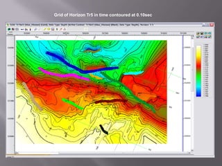
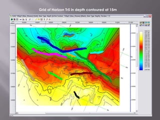
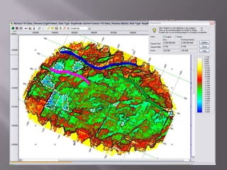
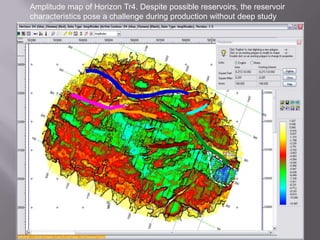
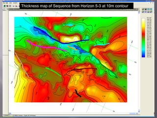
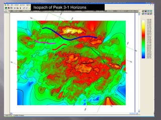
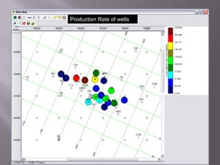
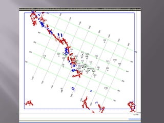
This document discusses applications of geographic information systems (GIS) including urban planning, 3D modeling, environmental analysis, and hydrocarbon exploration. It provides examples of how GIS has been used for urban planning tasks like siting a daycare, modeling population change, and analyzing transportation networks. 3D modeling applications include generating high-resolution digital models from laser scanning data for uses like mapping, education, and engineering. Environmental analysis examples include examining the relationship between toxic sites and disadvantaged communities. The document also discusses GIS applications in hydrocarbon exploration like mapping fields and reservoirs, seismic interpretation, and production analysis to optimize resource development.