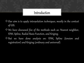
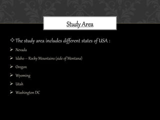
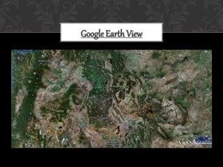
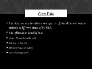
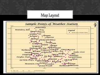
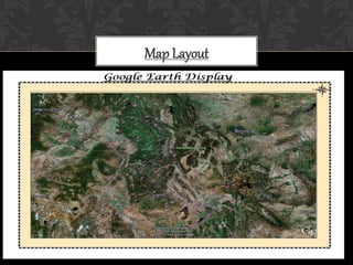
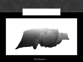
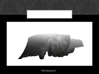
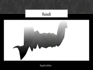
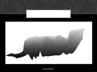
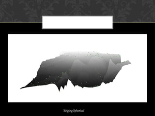
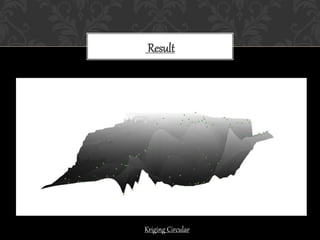
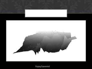
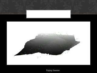
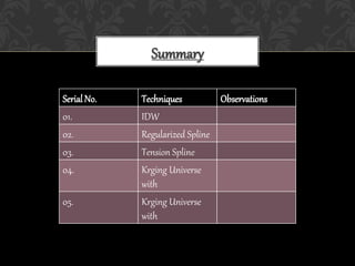
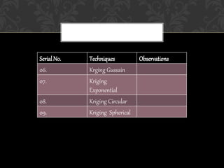
In context of Arc GIS
INTERPOLATION
TECHNIQUES
Our aim is to apply interpolation techniques, mostly in the context
of GIS.
We have discussed few of the methods such as: Nearest neighbor,
IDW, Spline, Radial Basis Function, and Kriging.
But we have done analysis on: IDW, Spline (tension and
registration) and Kriging (ordinary and universal).
Introduction
The study area includes different states of USA :
 Nevada
 Idaho – Rocky Mountains (side of Montana)
 Oregon
 Wyoming
 Utah
 Washington DC
Study Area
Google Earth View
The data we use to achieve our goal is of the different weather
stations in different states of the USA.
The information it includes is:
 Station Names (in text format)
 Lat/long (in degress)
 Elevation Values (in meters)
 Rain Percentage (in %)
Given Data
Map Layout
Map Layout
 The method which we adopt here is the technique of Interpolation
data from sample points.
 As defined earlier, the software that aid us is the Arc GIS and Arc
Scene (version 9.3) .
 Different types of interpolation techniques gives us separate
results.
 As we display the sample points on Arc GIS, and also label them.
 We interpolate data using the attribute of Elevation field. (others
can also be used).
Methodology
Literature Review
Interpolating A Surface fromSample Point Data
Interpolation
Estimating the attribute values of locations that are within the
range of available data using known data values.
Extrapolation
Estimating the attribute values of locations outside the range of
available data using known data values.
Interpolation
Extrapolation
Linear Interpolation
Elevation profile
Sample
elevation data
A
B
If
A = 8 feet and
B = 4 feet
then
C = (8 + 4) / 2 = 6 feet
C
Non-linear Interpolation
Elevation profile
Sample
elevation data
A
B
C
• Often results in a more
realistic interpolation
but estimating missing
data values is more
complex
Sampling
Strategy
Random
Regular
Sampling Strategies
Guarantees a good spread of points.
Regular Strategy
 It produces a pattern with clustering some areas.
RandomStrategy
Spatial Interpolation MethodsSpatialInterpolation
Methods
Global
Deterministic
Exact
Inexact
Geo-Statistical
Exact
Inexact
Local
Deterministic
Exact
Inexact
Geo-Statistical
Exact
Inexact
Global Interpolation
Sample
data
 Uses all Known Points to estimate a value at unsampled
locations.
 More generalize estimation.
 Useful for the terrains that do not show abrupt change.
Local Interpolation
Sample data
• Uses a local neighborhood to
estimate value, i.e. closest n
number of points, or within a given
search radius
 Uses a neighborhood of sample points to estimate the a value
at unsampled location.
 Produce local estimation.
 Useful for abrupt changes.
Grouping of Interpolation
Grouping
Deterministic
Geo-
Statistical
 Deterministic interpolation techniques create surfaces
from measured points.
 A deterministic interpolation can either force the resulting
surface to pass through the data values or not.
Deterministic Technique
 Geo-statistical techniques quantify the spatial
autocorrelation among measured points and account for
the spatial configuration of the sample points around the
prediction location.
 Because geo-statistics is based on statistics, these
techniques produce not only prediction surfaces but also
error or uncertainty surfaces, giving you an indication of
how good the predictions are
Geo-statistical Technique
Exact Interpolation: predicts a value that is identical to the
measured value at a sampled location.
Inexact interpolator: predicts a value that is different from the
measured value
Examples
Nearest Neighbor(NN)
Predicts the value on the basis of the perpendicular bisector between
sampled points forming Thiession Polygons.
Produces 1 polygon per sample point,
With sample point at the center.
It weights as per the area or the volume.
They are further divided into two more
categories.
 It is Local, Deterministic, and Exact.
Inverse Distance Weighted(IDW)
It is advanced of Nearest Neighbor.
Here the driving force is Distance.
It includes ore observation other than the nearest points.
It is Local, Deterministic, and Exact.
With the high power, the surface get soother and smoother
Result
IDW with 8
IDW with power 2
IDW with power 4
IDW with power 8
Spline
Those points that are extended to the height of their magnitude
Act as bending of a rubber sheet while minimizing the curvature.
Can be used for the smoothing of the surface.
Surface passes from all points.
They can be 1st , 2nd , and 3rd order:
 Regular (1st, 2nd , & 3rd )
 Tension (1st , & 2nd )
They can 2D (smoothing a contour) or 3D (modeling a surface).
They can be Local, Deterministic, and Exact.
 Regularized Spline: the higher the weight, the smoother the surface.
 Typical values are: 0.1, 0.01, 0.001, 0.5 etc
 Suitable values are: 0-5.
 Tension Spline: the higher the weight, the coarser the surface.
 Must be greater than equal to zero
 Typical values are: 0, 1, 5, 10.
Result
Regular Spline
Tension Spline
 The number of point are set by default in most of the software.
 The number of points one define, all the number are used in the
calculation
 Maximum the number, smoother the surface.
 Lesser the stiffness.
Radial Basis Function (RBS)
Is a function that changes its location with distance.
It can predicts a value above the maximum and below the
minimum
Basically, it is the series of exact interpolation techniques:
 Thin-plate Spline
 Spline with Tension
 Regularized Spline
 Multi-Quadratic Function
 Inverse Multi-quadratic Spline
Trend Surface
 Produces surface that represents gradual trend over area of
interest.
 It is Local, Estimated, and Geo-statistical.
 Examining or removing the long range trends.
 1st Order
 2nd Order
Kirging
 It says that the distance and direction between sample points
shows the spatial correlation that can be used to predict the
surface
 Merits: it is fast and flexible method.
 Demerit: requires a lot of decision making
 In Kriging, the weight not only depends upon the distance of the
measured and prediction points, but also on the spatial
arrangement of them.
 It uses data twice:
 To estimate the spatial correlation, and
 To make the predictions
 Ordinary Kriging: Suitable for the data having trend. (e.g.
mountains along with valleys)
 Computed with constant mean “µ”
 Universal Kriging: The results are similar to the one get from
regression.
 Sample points arrange themselves above and below the mean.
 More like a 2nd order polynomial.
Result
Ordinary Kriging
Universal Kriging
 It quantifies the assumption that nearby things tend to be more
similar than that are further apart.
 It measures the statistical correlation.
 It shows that greater the distance between two points, lesser the
similarity between them.
Semi-variogram
It can be:
 Spherical
 Circular
 Exponential
 Gaussian
Kriging Spherical
Result
Kriging Circular
Kriging Exponential
Kriging Gaussian
Summary
Serial No. Techniques Observations
01. IDW
02. Regularized Spline
03. Tension Spline
04. Krging Universe
with
05. Krging Universe
with
Serial No. Techniques Observations
06. Krging Gussain
07. Kriging
Exponential
08. Kriging Circular
09. Kriging Spherical
 The final outcome of our experimentation is :
Conclusion

Interpolation 2013

  • 1.
    In context ofArc GIS INTERPOLATION TECHNIQUES
  • 2.
    Our aim isto apply interpolation techniques, mostly in the context of GIS. We have discussed few of the methods such as: Nearest neighbor, IDW, Spline, Radial Basis Function, and Kriging. But we have done analysis on: IDW, Spline (tension and registration) and Kriging (ordinary and universal). Introduction
  • 3.
    The study areaincludes different states of USA :  Nevada  Idaho – Rocky Mountains (side of Montana)  Oregon  Wyoming  Utah  Washington DC Study Area
  • 4.
  • 5.
    The data weuse to achieve our goal is of the different weather stations in different states of the USA. The information it includes is:  Station Names (in text format)  Lat/long (in degress)  Elevation Values (in meters)  Rain Percentage (in %) Given Data
  • 6.
  • 7.
  • 8.
     The methodwhich we adopt here is the technique of Interpolation data from sample points.  As defined earlier, the software that aid us is the Arc GIS and Arc Scene (version 9.3) .  Different types of interpolation techniques gives us separate results.  As we display the sample points on Arc GIS, and also label them.  We interpolate data using the attribute of Elevation field. (others can also be used). Methodology
  • 9.
  • 10.
    Interpolating A SurfacefromSample Point Data Interpolation Estimating the attribute values of locations that are within the range of available data using known data values. Extrapolation Estimating the attribute values of locations outside the range of available data using known data values.
  • 11.
  • 12.
  • 13.
    Linear Interpolation Elevation profile Sample elevationdata A B If A = 8 feet and B = 4 feet then C = (8 + 4) / 2 = 6 feet C
  • 14.
    Non-linear Interpolation Elevation profile Sample elevationdata A B C • Often results in a more realistic interpolation but estimating missing data values is more complex
  • 15.
  • 16.
    Guarantees a goodspread of points. Regular Strategy
  • 17.
     It producesa pattern with clustering some areas. RandomStrategy
  • 18.
  • 19.
    Global Interpolation Sample data  Usesall Known Points to estimate a value at unsampled locations.  More generalize estimation.  Useful for the terrains that do not show abrupt change.
  • 20.
    Local Interpolation Sample data •Uses a local neighborhood to estimate value, i.e. closest n number of points, or within a given search radius  Uses a neighborhood of sample points to estimate the a value at unsampled location.  Produce local estimation.  Useful for abrupt changes.
  • 21.
  • 22.
     Deterministic interpolationtechniques create surfaces from measured points.  A deterministic interpolation can either force the resulting surface to pass through the data values or not. Deterministic Technique
  • 23.
     Geo-statistical techniquesquantify the spatial autocorrelation among measured points and account for the spatial configuration of the sample points around the prediction location.  Because geo-statistics is based on statistics, these techniques produce not only prediction surfaces but also error or uncertainty surfaces, giving you an indication of how good the predictions are Geo-statistical Technique
  • 24.
    Exact Interpolation: predictsa value that is identical to the measured value at a sampled location.
  • 25.
    Inexact interpolator: predictsa value that is different from the measured value
  • 26.
  • 27.
    Nearest Neighbor(NN) Predicts thevalue on the basis of the perpendicular bisector between sampled points forming Thiession Polygons. Produces 1 polygon per sample point, With sample point at the center. It weights as per the area or the volume. They are further divided into two more categories.  It is Local, Deterministic, and Exact.
  • 28.
    Inverse Distance Weighted(IDW) Itis advanced of Nearest Neighbor. Here the driving force is Distance. It includes ore observation other than the nearest points. It is Local, Deterministic, and Exact. With the high power, the surface get soother and smoother
  • 29.
  • 30.
  • 31.
  • 32.
    Spline Those points thatare extended to the height of their magnitude Act as bending of a rubber sheet while minimizing the curvature. Can be used for the smoothing of the surface. Surface passes from all points. They can be 1st , 2nd , and 3rd order:  Regular (1st, 2nd , & 3rd )  Tension (1st , & 2nd ) They can 2D (smoothing a contour) or 3D (modeling a surface). They can be Local, Deterministic, and Exact.
  • 33.
     Regularized Spline:the higher the weight, the smoother the surface.  Typical values are: 0.1, 0.01, 0.001, 0.5 etc  Suitable values are: 0-5.  Tension Spline: the higher the weight, the coarser the surface.  Must be greater than equal to zero  Typical values are: 0, 1, 5, 10.
  • 34.
  • 35.
  • 36.
     The numberof point are set by default in most of the software.  The number of points one define, all the number are used in the calculation  Maximum the number, smoother the surface.  Lesser the stiffness.
  • 37.
    Radial Basis Function(RBS) Is a function that changes its location with distance. It can predicts a value above the maximum and below the minimum Basically, it is the series of exact interpolation techniques:  Thin-plate Spline  Spline with Tension  Regularized Spline  Multi-Quadratic Function  Inverse Multi-quadratic Spline
  • 38.
    Trend Surface  Producessurface that represents gradual trend over area of interest.  It is Local, Estimated, and Geo-statistical.  Examining or removing the long range trends.  1st Order  2nd Order
  • 39.
    Kirging  It saysthat the distance and direction between sample points shows the spatial correlation that can be used to predict the surface  Merits: it is fast and flexible method.  Demerit: requires a lot of decision making
  • 40.
     In Kriging,the weight not only depends upon the distance of the measured and prediction points, but also on the spatial arrangement of them.  It uses data twice:  To estimate the spatial correlation, and  To make the predictions
  • 41.
     Ordinary Kriging:Suitable for the data having trend. (e.g. mountains along with valleys)  Computed with constant mean “µ”  Universal Kriging: The results are similar to the one get from regression.  Sample points arrange themselves above and below the mean.  More like a 2nd order polynomial.
  • 42.
  • 43.
  • 44.
     It quantifiesthe assumption that nearby things tend to be more similar than that are further apart.  It measures the statistical correlation.  It shows that greater the distance between two points, lesser the similarity between them. Semi-variogram
  • 45.
    It can be: Spherical  Circular  Exponential  Gaussian
  • 46.
  • 47.
  • 48.
  • 49.
  • 50.
    Summary Serial No. TechniquesObservations 01. IDW 02. Regularized Spline 03. Tension Spline 04. Krging Universe with 05. Krging Universe with
  • 51.
    Serial No. TechniquesObservations 06. Krging Gussain 07. Kriging Exponential 08. Kriging Circular 09. Kriging Spherical
  • 52.
     The finaloutcome of our experimentation is : Conclusion