Download to read offline


![Summary of Statistical Problem
Goal: Learn about θ based on two sources of information:
Observations:
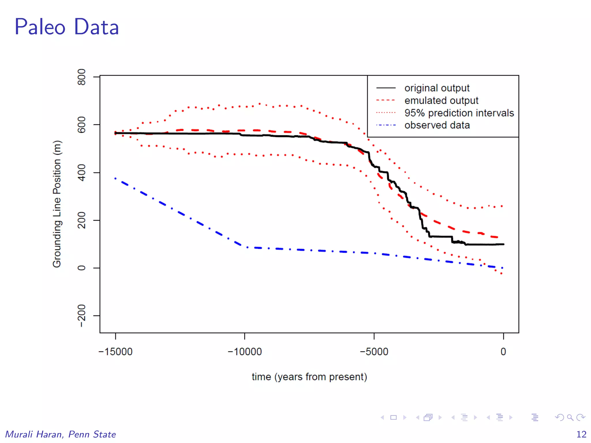
1. Observed time series of past grounding line positions
reconstructed from paleo records: Z1 = (Z1(t1), . . . , Z1(tn))T
,
t1, . . . , tn are time points locations.
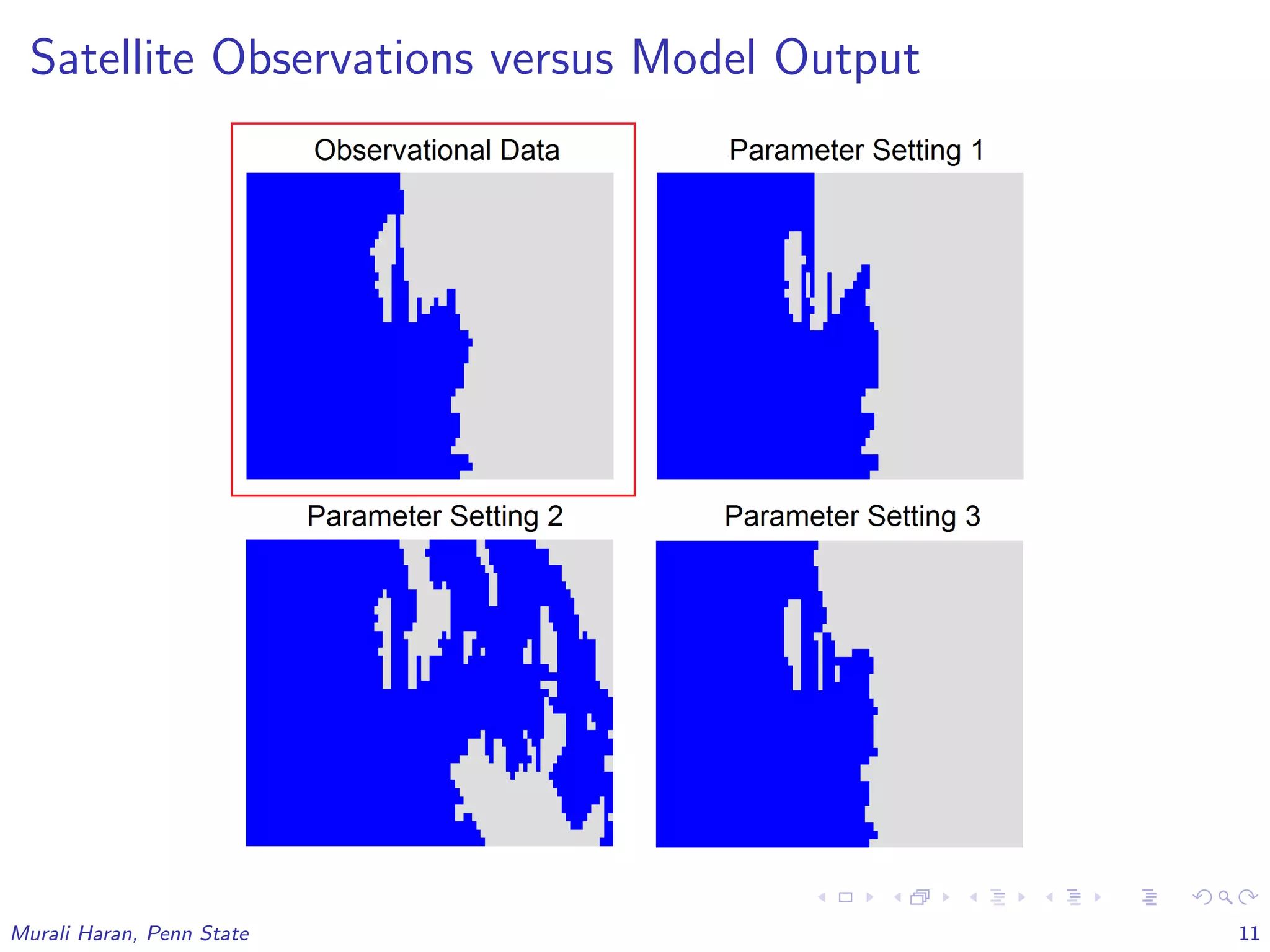
2. Observed modern ice-no ice from satellite data:
Z2 = [Z2(s1), . . . , Z2(sm)], locations s1, . . . , sm.
Model output
1. Y1(θ1), . . . , Y1(θp), where each
Y1(θi ) = (Y1(θi , t1), . . . , Y1(θi , tn))T
is a time series of
grounding line positions at parameter setting θi .
2. Y2(θ1), . . . , Y2(θp), where each
Y2(θi ) = (Y2(θi , s1), . . . , Y2(θi , sm))T
is a vector of spatial
data at parameter setting θi .
Murali Haran, Penn State 17](https://image.slidesharecdn.com/statchallengesharan-170827232548/75/Program-on-Mathematical-and-Statistical-Methods-for-Climate-and-the-Earth-System-Opening-Workshop-Some-Statistical-Challenges-in-Studying-the-West-Antarctic-Ice-Sheet-Murali-Haran-Aug-22-2017-17-2048.jpg)
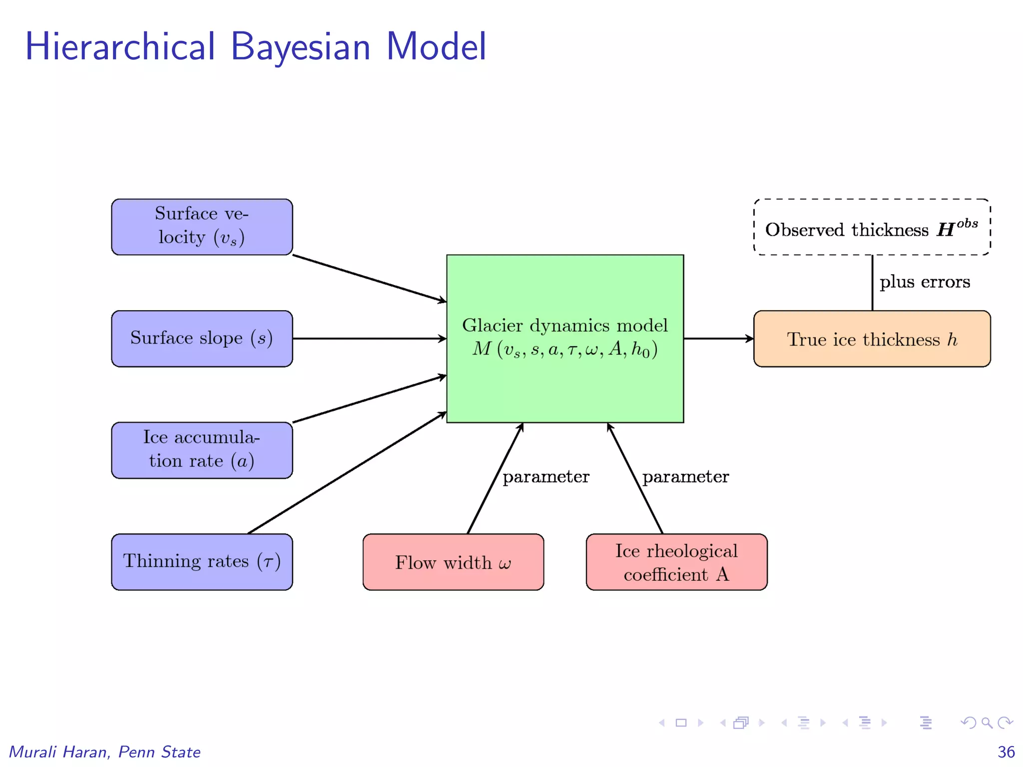


The document discusses the statistical challenges in studying the West Antarctic Ice Sheet, emphasizing the importance of understanding ice sheet dynamics and making accurate projections of ice behavior to assess potential sea level rise. It outlines the use of sophisticated statistical methods, including model emulation and calibration, to infer parameters and bridge data discrepancies in ice sheet modeling. The work also highlights the need for integrating multiple data sources to improve the accuracy of projections related to ice streams and overall ice sheet stability.