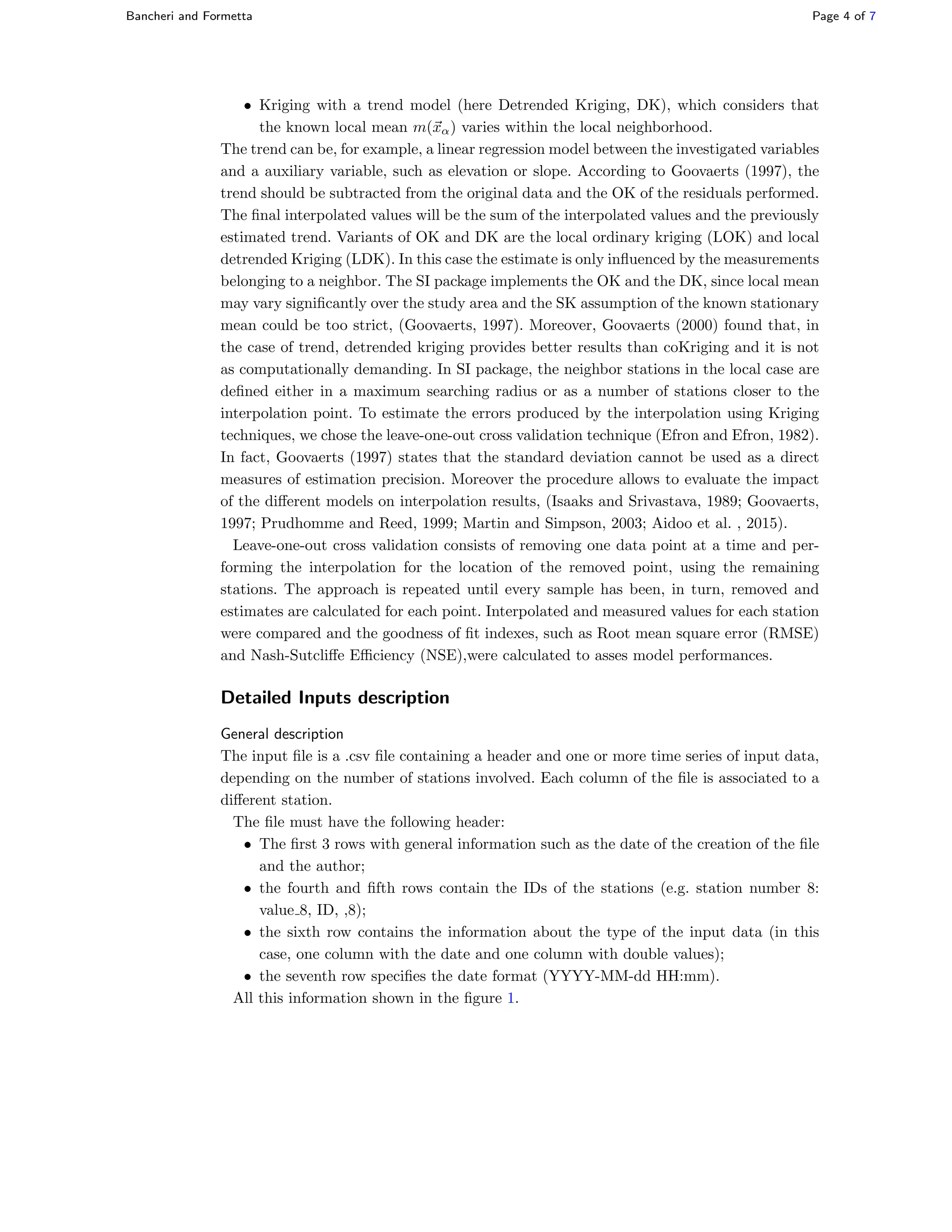
SlideShare a Scribd company logo
Bancheri and Formetta
LINKERS
JGrass-NewAGE: Kriging component
Marialaura Bancheri*†
and Giuseppe Formetta†
*
Correspondence:
marialaura.bancheri@unitn.it
Dipartimento di Ingegneria Civile
Ambientale e Meccanica, Trento,
Mesiano di Povo, Trento, IT
Full list of author information is
available at the end of the article
†
Code Author
Abstract
These pages teach how to run the Kriging component inside the OMS 3 console.
Some preliminary knowledge and installation of OMS is mandatory (see @Also useful).
This component deals with the interpolation of the spatial behavior of climatological
variable following the approach proposed by Matheron (1981) and Goovaerts (1997). It
implements 10 theoretical semivariogram models and 4 types of Kriging algorithms, for
a total of forty interpolation options. The component can be used with both raster
inputs and punctual inputs. It is perfectly integrated in the system and its outputs can
be the inputs of different components.
@Version:
0.1
@License:
GPL v. 3
@Inputs:
• Climatological variable (−);
• Shapefile of the weather station, containing also the elevation information (m)
required for detrended kriging (DK);
• Shapefile of the sub-basin centroid containing also the elevation information (m)
required for detrended kriging (DK);
• Start date (String);
• End date (String);
• number of station the algorithm has to consider;
• range (m);
• sill (−);
• nugget (−);
• type of the semivariogram to use (String);
@Outputs:
• Climatological variable interpolated (−);
@Doc Author: Marialaura Bancheri
@References:
• See References section below
Keywords: OMS; JGrass-NewAGE Component Description; Kriging
Bancheri and Formetta Page 2 of 7
Code Information
Executables
This link points to the jar file that, once downloaded can be used in the OMS console:
https://github.com/GEOframeOMSProjects/OMS_Project_Krigings/tree/master/
lib
Developer Info
This link points to useful information for the developers, i.e. information about the code
internals, algorithms and the source code
https://github.com/geoframecomponents
Also useful
To run JGrass-NewAGE it is necessary to know how to use the OMS console. Information
at: ”How to install and run the OMS console”,
https://alm.engr.colostate.edu/cb/project/oms).
JGrasstools are required for preparing some input data (information at:
http://abouthydrology.blogspot.it/2012/11/udig-jgrasstools-resources-in-italian.
html
To visualize results you need a GIS. Use your preferred GIS, following its installation
instructions. To make statistics on the results, you can probably get benefits from R:
http://www.r-project.org/ and follow its installation instruction.
To whom address questions
marialaura.bancheri@unitn.it
Authors of documentation
Marialaura Bancheri (marialaura.bancheri@unitn.it)
This documentation is released under Creative Commons 4.0 Attribution International
Bancheri and Formetta Page 3 of 7
Component Description
Kriging is a group of geostatistical techniques used to interpolate the value of random
fields based on spatial autocorrelation of measured data (1, Chapter 6.2). The measure-
ments value z(xα) and the unknown value z(x), where x is the location, given according
to a certain cartographic projection, are considered as particular realizations of random
variables Z(xα) and Z(x) (Goovaerts, 1997; Isaaks and Srivastava, 1989). The estimation
of the unknown value zλ
(x), where the true unknown value is Zλ
(x), is obtained as a
linear combination of the N values at surrounding points, Goovaerts (1999):
Zλ
(x) − m(x) =
N
α=1
λ(xα)[Z(uα) − m(xα)] (1)
where m(x) and m(xα) are the expected values of the random variables Z(x) and Z(xα).
λ(xα) is the weight assigned to datum z(xα). Weights are chosen to satisfy the conditions
of minimizing the error of variance of the estimator σ2
λ, that is:
argmin
λ
σ2
λ ≡ argmin
λ
VarZλ
(x) − Z(x) (2)
under the constrain that the estimate is unbiased, i.e.
EZλ
(x) − Z(x) = 0 (3)
The latter condition, implies that:
N
α=1
λα(xα) = 1 (4)
As shown in various textbooks, e.g. Kitanidis (1997), the above conditions bring to a linear
system whose unknown is the tuple of weights, and the system matrix depends on the
semivariograms among the couples of the known sites. When it is made the assumption
of isotropy of the spatial statistics of the quantity analyzed, the semivariogram is given
by Cressie and Cassie (1993):
γ(h) :=
1
2Nh
Nh
i=1
(Z(x) − Z(x)i)2
(5)
where the distance (x, xi) ≡ h, Nh denotes the set of pairs of observations at local x and
at location xi at distance h apart from x. In order to be extended to any distance, ex-
perimental semivariogram need to be fitted to a theoretical semivariogram model. These
theoretical semivariograms contain parameters (called nugget, sill and range) to be fitted
against the existing data, before introducing in the Kriging linear system, whose solu-
tion returns the weights in eq.(1). Three main variants of Kriging can be distinguished,
(Goovaerts, 1997):
• Simple Kriging (SK),which considers the mean, m(x), to be known and constant
throughout the study area;
• Ordinary Kriging (OK) ,which account for local fluctuations of the mean, limiting
the stationarity to the local neighborhood. In this case, the mean in unknown.
Bancheri and Formetta Page 4 of 7
• Kriging with a trend model (here Detrended Kriging, DK), which considers that
the known local mean m(xα) varies within the local neighborhood.
The trend can be, for example, a linear regression model between the investigated variables
and a auxiliary variable, such as elevation or slope. According to Goovaerts (1997), the
trend should be subtracted from the original data and the OK of the residuals performed.
The final interpolated values will be the sum of the interpolated values and the previously
estimated trend. Variants of OK and DK are the local ordinary kriging (LOK) and local
detrended Kriging (LDK). In this case the estimate is only influenced by the measurements
belonging to a neighbor. The SI package implements the OK and the DK, since local mean
may vary significantly over the study area and the SK assumption of the known stationary
mean could be too strict, (Goovaerts, 1997). Moreover, Goovaerts (2000) found that, in
the case of trend, detrended kriging provides better results than coKriging and it is not
as computationally demanding. In SI package, the neighbor stations in the local case are
defined either in a maximum searching radius or as a number of stations closer to the
interpolation point. To estimate the errors produced by the interpolation using Kriging
techniques, we chose the leave-one-out cross validation technique (Efron and Efron, 1982).
In fact, Goovaerts (1997) states that the standard deviation cannot be used as a direct
measures of estimation precision. Moreover the procedure allows to evaluate the impact
of the different models on interpolation results, (Isaaks and Srivastava, 1989; Goovaerts,
1997; Prudhomme and Reed, 1999; Martin and Simpson, 2003; Aidoo et al. , 2015).
Leave-one-out cross validation consists of removing one data point at a time and per-
forming the interpolation for the location of the removed point, using the remaining
stations. The approach is repeated until every sample has been, in turn, removed and
estimates are calculated for each point. Interpolated and measured values for each station
were compared and the goodness of fit indexes, such as Root mean square error (RMSE)
and Nash-Sutcliffe Efficiency (NSE),were calculated to asses model performances.
Detailed Inputs description
General description
The input file is a .csv file containing a header and one or more time series of input data,
depending on the number of stations involved. Each column of the file is associated to a
different station.
The file must have the following header:
• The first 3 rows with general information such as the date of the creation of the file
and the author;
• the fourth and fifth rows contain the IDs of the stations (e.g. station number 8:
value 8, ID, ,8);
• the sixth row contains the information about the type of the input data (in this
case, one column with the date and one column with double values);
• the seventh row specifies the date format (YYYY-MM-dd HH:mm).
All this information shown in the figure 1.
Bancheri and Formetta Page 5 of 7
Figure 1 Heading of the .csv input file
Total precipitation
The total precipitation is given in time series or raster maps of (mm) values.
Relative humidity
The relative humidity is given in time series or raster maps of (%) values.
Air temperature
The air temperature is given in time series or raster maps of (◦
C) values.
range
range is the distance after which data are no longer correlated.
sill
sill is the total variance where the empirical variogram appears to level off.
nugget
nugget is related to the amount of short range variability in the data. A nugget that’s
large relative to the sill is problematic and could indicate too much noise and not enough
spatial correlation
semivariogram
semivariogram describes the degree of spatial dependence of the climatological variable.
Detailed Outputs description
Climatological variable
The interpolated climatological variable is given as a time series at each sub-basin centroid
Examples
The following .sim file is customized for the use of the kriging component. The .sim file
can be downloaded from here:
https://github.com/GEOframeOMSProjects/OMS_Project_Krigings/tree/master/
simulation
import static oms3.SimBuilder.instance as OMS3
def home = oms_prj
// start and end date of the simulation
def startDate= "2000 -01 -01 00:00"
def endDate="2000 -01 -01 00:00"
Bancheri and Formetta Page 6 of 7
OMS3.sim {
resource "$oms_prj/lib"
model(while: "reader_data.doProcess" ) {
components {
// components to be called : reader input data , lwrb and writer
output data
" reader_data " org. jgrasstools .gears.io. timedependent .
OmsTimeSeriesIteratorReader "
" vreader_station " "org.jgrasstools.gears.io.shapefile.
OmsShapefileFeatureReader "
// comment this component if you want to use the ordinary Kriging
"trend" " trendAnalysis . TrendAnalysis "
" vreader_interpolation " "org.jgrasstools.gears.io.shapefile.
OmsShapefileFeatureReader "
"kriging" "krigings.Krigings"
" writer_interpolated " "org. jgrasstools.gears.io. timedependent .
OmsTimeSeriesIteratorWriter "
}
parameter{
" reader_data .file" "${home }/ data/rain_test.csv"
" reader_data .idfield" "ID"
" reader_data .tStart" "${startDate}"
" reader_data .tEnd" "${endDate}"
" reader_data .tTimestep" 60
" reader_data .fileNovalue" " -9999"
" vreader_station .file" "${home }/ data/ rainstations .shp"
" vreader_interpolation .file" "${home }/ data/
basins_passirio_width0 .shp"
// comment this line if you want to use the ordinary Kriging
"trend. fStationsid " "ID_PUNTI_M"
// comment this line if you want to use the ordinary Kriging
"trend.fStationsZ" "QUOTA"
// comment this line if you want to use the ordinary Kriging
"trend. thresholdCorrelation " 0
"kriging.fStationsid" "ID_PUNTI_M"
"kriging. fInterpolateid " "netnum"
"kriging. inNumCloserStations " 5
"kriging.range" 123537.0
"kriging.nugget" 0.0
"kriging.sill" 1.678383
// parameter of the writing component
" writer_interpolated .file" "${home }/ output/
kriging_detrendend .csv"
" writer_interpolated .tStart" "${startDate}"
" writer_interpolated .tTimestep" 60
}
connect {
// if you want to use the ordinary Kriging uncomment this line
// " reader_data .outData" "kriging.inData"
// comment this line if you want to use the ordinary Kriging
" reader_data .outData" "trend.inData"
// comment this line if you want to use the ordinary Kriging
" vreader_station .geodata" "trend.inStations"
Bancheri and Formetta Page 7 of 7
" vreader_station .geodata" "kriging.inStations"
" vreader_interpolation .geodata" "kriging. inInterpolate "
// comment this line if you want to use the ordinary Kriging
"trend. outResiduals " "kriging.inData"
// comment this line if you want to use the ordinary Kriging
"trend. trend_intercept " "kriging. trend_intercept "
// comment this line if you want to use the ordinary Kriging
"trend. trend_coefficient " "kriging. trend_coefficient "
// comment this line if you want to use the ordinary Kriging
"trend. doDetrended " "kriging.doDetrended"
"kriging.outData" " writer_interpolated .inData"
}
}
}
Data and Project
The following link is for the download of the input data necessaries to execute the CI
component (as shown in the .sim file in the previous section ) :
https://github.com/GEOframeOMSProjects/OMS_Project_Krigings/tree/master/
data
The following link is for the download of the OMS project for the component:
https://github.com/GEOframeOMSProjects/OMS_Project_Krigings
%
References
1. Bancheri, M.: A flexible approach to the estimation of water budgets and its connection to the travel time theory. PhD
thesis, Universit`a degli Studi di Trento (2017)

More Related Content

What's hot

Pakdd
PakddPakdd
Pakdd
Siswanto .
 
Introduction geostatistic for_mineral_resources
Introduction geostatistic for_mineral_resourcesIntroduction geostatistic for_mineral_resources
Introduction geostatistic for_mineral_resources
Adi Handarbeni
 
Method of Fracture Surface Matching Based on Mathematical Statistics
Method of Fracture Surface Matching Based on Mathematical StatisticsMethod of Fracture Surface Matching Based on Mathematical Statistics
Method of Fracture Surface Matching Based on Mathematical Statistics
IJRESJOURNAL
 
Variograms
VariogramsVariograms
Variograms
ohn thaik
 
Evolution of 3D Surface Parameters: A Comprehensive Survey
Evolution of 3D Surface Parameters: A Comprehensive SurveyEvolution of 3D Surface Parameters: A Comprehensive Survey
Evolution of 3D Surface Parameters: A Comprehensive Survey
theijes
 
4 hydrology geostatistics-part_2
4 hydrology geostatistics-part_2 4 hydrology geostatistics-part_2
4 hydrology geostatistics-part_2
Riccardo Rigon
 
Spatial interpolation comparison
Spatial interpolation comparisonSpatial interpolation comparison
Spatial interpolation comparison
Tomislav Hengl
 
Basics1variogram
Basics1variogramBasics1variogram
Basics1variogram
Robert Lopez
 
Numerical disperison analysis of sympletic and adi scheme
Numerical disperison analysis of sympletic and adi schemeNumerical disperison analysis of sympletic and adi scheme
Numerical disperison analysis of sympletic and adi schemexingangahu
 
Concurrent Ternary Galois-based Computation using Nano-apex Multiplexing Nibs...
Concurrent Ternary Galois-based Computation using Nano-apex Multiplexing Nibs...Concurrent Ternary Galois-based Computation using Nano-apex Multiplexing Nibs...
Concurrent Ternary Galois-based Computation using Nano-apex Multiplexing Nibs...
VLSICS Design
 
ENHANCEMENT OF TRANSMISSION RANGE ASSIGNMENT FOR CLUSTERED WIRELESS SENSOR NE...
ENHANCEMENT OF TRANSMISSION RANGE ASSIGNMENT FOR CLUSTERED WIRELESS SENSOR NE...ENHANCEMENT OF TRANSMISSION RANGE ASSIGNMENT FOR CLUSTERED WIRELESS SENSOR NE...
ENHANCEMENT OF TRANSMISSION RANGE ASSIGNMENT FOR CLUSTERED WIRELESS SENSOR NE...
IJCNCJournal
 
Student_Garden_geostatistics_course
Student_Garden_geostatistics_courseStudent_Garden_geostatistics_course
Student_Garden_geostatistics_coursePedro Correia
 
Trajectory clustering - Traclus Algorithm
Trajectory clustering - Traclus AlgorithmTrajectory clustering - Traclus Algorithm
Trajectory clustering - Traclus Algorithm
Iván Sanchez Vera
 
A Subgraph Pattern Search over Graph Databases
A Subgraph Pattern Search over Graph DatabasesA Subgraph Pattern Search over Graph Databases
A Subgraph Pattern Search over Graph Databases
IJMER
 
Ch11.kriging
Ch11.krigingCh11.kriging
Ch11.kriging
Ajay Mishra
 
Geographical information system
Geographical  information systemGeographical  information system
Geographical information system
Satya Prakash Dalei
 

What's hot (20)

Pakdd
PakddPakdd
Pakdd
 
Introduction geostatistic for_mineral_resources
Introduction geostatistic for_mineral_resourcesIntroduction geostatistic for_mineral_resources
Introduction geostatistic for_mineral_resources
 
Method of Fracture Surface Matching Based on Mathematical Statistics
Method of Fracture Surface Matching Based on Mathematical StatisticsMethod of Fracture Surface Matching Based on Mathematical Statistics
Method of Fracture Surface Matching Based on Mathematical Statistics
 
Variograms
VariogramsVariograms
Variograms
 
Evolution of 3D Surface Parameters: A Comprehensive Survey
Evolution of 3D Surface Parameters: A Comprehensive SurveyEvolution of 3D Surface Parameters: A Comprehensive Survey
Evolution of 3D Surface Parameters: A Comprehensive Survey
 
4 hydrology geostatistics-part_2
4 hydrology geostatistics-part_2 4 hydrology geostatistics-part_2
4 hydrology geostatistics-part_2
 
Spatial interpolation comparison
Spatial interpolation comparisonSpatial interpolation comparison
Spatial interpolation comparison
 
Basics1variogram
Basics1variogramBasics1variogram
Basics1variogram
 
Numerical disperison analysis of sympletic and adi scheme
Numerical disperison analysis of sympletic and adi schemeNumerical disperison analysis of sympletic and adi scheme
Numerical disperison analysis of sympletic and adi scheme
 
Snow tra 3d
Snow tra 3dSnow tra 3d
Snow tra 3d
 
Concurrent Ternary Galois-based Computation using Nano-apex Multiplexing Nibs...
Concurrent Ternary Galois-based Computation using Nano-apex Multiplexing Nibs...Concurrent Ternary Galois-based Computation using Nano-apex Multiplexing Nibs...
Concurrent Ternary Galois-based Computation using Nano-apex Multiplexing Nibs...
 
Hsieh etal spl
Hsieh etal splHsieh etal spl
Hsieh etal spl
 
ENHANCEMENT OF TRANSMISSION RANGE ASSIGNMENT FOR CLUSTERED WIRELESS SENSOR NE...
ENHANCEMENT OF TRANSMISSION RANGE ASSIGNMENT FOR CLUSTERED WIRELESS SENSOR NE...ENHANCEMENT OF TRANSMISSION RANGE ASSIGNMENT FOR CLUSTERED WIRELESS SENSOR NE...
ENHANCEMENT OF TRANSMISSION RANGE ASSIGNMENT FOR CLUSTERED WIRELESS SENSOR NE...
 
Final Report
Final ReportFinal Report
Final Report
 
Dkd 4 2-sheet_1_annex_a
Dkd 4 2-sheet_1_annex_aDkd 4 2-sheet_1_annex_a
Dkd 4 2-sheet_1_annex_a
 
Student_Garden_geostatistics_course
Student_Garden_geostatistics_courseStudent_Garden_geostatistics_course
Student_Garden_geostatistics_course
 
Trajectory clustering - Traclus Algorithm
Trajectory clustering - Traclus AlgorithmTrajectory clustering - Traclus Algorithm
Trajectory clustering - Traclus Algorithm
 
A Subgraph Pattern Search over Graph Databases
A Subgraph Pattern Search over Graph DatabasesA Subgraph Pattern Search over Graph Databases
A Subgraph Pattern Search over Graph Databases
 
Ch11.kriging
Ch11.krigingCh11.kriging
Ch11.kriging
 
Geographical information system
Geographical  information systemGeographical  information system
Geographical information system
 

Similar to Jgrass-NewAge: Kriging component

JGrass-Newage SWRB
JGrass-Newage SWRBJGrass-Newage SWRB
JGrass-Newage SWRB
Marialaura Bancheri
 
Air quality dispersion modeling
Air quality dispersion modelingAir quality dispersion modeling
Air quality dispersion modeling
ECRD IN
 
Numerical simulaton of axial flow fan using gambit and
Numerical simulaton of axial flow fan using gambit andNumerical simulaton of axial flow fan using gambit and
Numerical simulaton of axial flow fan using gambit and
eSAT Publishing House
 
Lwrb ms
Lwrb msLwrb ms
SVD BASED LATENT SEMANTIC INDEXING WITH USE OF THE GPU COMPUTATIONS
SVD BASED LATENT SEMANTIC INDEXING WITH USE OF THE GPU COMPUTATIONSSVD BASED LATENT SEMANTIC INDEXING WITH USE OF THE GPU COMPUTATIONS
SVD BASED LATENT SEMANTIC INDEXING WITH USE OF THE GPU COMPUTATIONS
ijscmcj
 
Choice of Numerical Integration Method for Wind Time History Analysis of Tall...
Choice of Numerical Integration Method for Wind Time History Analysis of Tall...Choice of Numerical Integration Method for Wind Time History Analysis of Tall...
Choice of Numerical Integration Method for Wind Time History Analysis of Tall...
inventy
 
A Novel Technique in Software Engineering for Building Scalable Large Paralle...
A Novel Technique in Software Engineering for Building Scalable Large Paralle...A Novel Technique in Software Engineering for Building Scalable Large Paralle...
A Novel Technique in Software Engineering for Building Scalable Large Paralle...
Eswar Publications
 
How to Decide the Best Fuzzy Model in ANFIS
How to Decide the Best Fuzzy Model in ANFIS How to Decide the Best Fuzzy Model in ANFIS
JGrass-NewAge LongWave radiation Balance
JGrass-NewAge LongWave radiation BalanceJGrass-NewAge LongWave radiation Balance
JGrass-NewAge LongWave radiation Balance
Marialaura Bancheri
 
SD-GCM Formulas
SD-GCM FormulasSD-GCM Formulas
SD-GCM Formulas
Sohrab Kolsoumi
 
Path Loss Prediction by Robust Regression Methods
Path Loss Prediction by Robust Regression MethodsPath Loss Prediction by Robust Regression Methods
Path Loss Prediction by Robust Regression Methods
ijceronline
 
Inversão com sigmoides
Inversão com sigmoidesInversão com sigmoides
Inversão com sigmoides
juarezsa
 
Adige modelling
Adige modellingAdige modelling
Colombo14a
Colombo14aColombo14a
Colombo14a
AlferoSimona
 
Field Strength Predicting Outdoor Models
Field Strength Predicting Outdoor ModelsField Strength Predicting Outdoor Models
Field Strength Predicting Outdoor Models
IRJET Journal
 
CVS vs. t2 -x 2 velocity analysis
CVS vs. t2 -x 2 velocity analysisCVS vs. t2 -x 2 velocity analysis
CVS vs. t2 -x 2 velocity analysis
iosrjce
 
JGrass-Newage snow component
JGrass-Newage snow componentJGrass-Newage snow component
JGrass-Newage snow component
Marialaura Bancheri
 
Dycops2019
Dycops2019 Dycops2019
Dycops2019
Jéssyca Bessa
 
Economia01
Economia01Economia01
Economia01
Crist Oviedo
 

Similar to Jgrass-NewAge: Kriging component (20)

JGrass-Newage SWRB
JGrass-Newage SWRBJGrass-Newage SWRB
JGrass-Newage SWRB
 
Air quality dispersion modeling
Air quality dispersion modelingAir quality dispersion modeling
Air quality dispersion modeling
 
Numerical simulaton of axial flow fan using gambit and
Numerical simulaton of axial flow fan using gambit andNumerical simulaton of axial flow fan using gambit and
Numerical simulaton of axial flow fan using gambit and
 
Lwrb ms
Lwrb msLwrb ms
Lwrb ms
 
SVD BASED LATENT SEMANTIC INDEXING WITH USE OF THE GPU COMPUTATIONS
SVD BASED LATENT SEMANTIC INDEXING WITH USE OF THE GPU COMPUTATIONSSVD BASED LATENT SEMANTIC INDEXING WITH USE OF THE GPU COMPUTATIONS
SVD BASED LATENT SEMANTIC INDEXING WITH USE OF THE GPU COMPUTATIONS
 
Choice of Numerical Integration Method for Wind Time History Analysis of Tall...
Choice of Numerical Integration Method for Wind Time History Analysis of Tall...Choice of Numerical Integration Method for Wind Time History Analysis of Tall...
Choice of Numerical Integration Method for Wind Time History Analysis of Tall...
 
A Novel Technique in Software Engineering for Building Scalable Large Paralle...
A Novel Technique in Software Engineering for Building Scalable Large Paralle...A Novel Technique in Software Engineering for Building Scalable Large Paralle...
A Novel Technique in Software Engineering for Building Scalable Large Paralle...
 
How to Decide the Best Fuzzy Model in ANFIS
How to Decide the Best Fuzzy Model in ANFIS How to Decide the Best Fuzzy Model in ANFIS
How to Decide the Best Fuzzy Model in ANFIS
 
JGrass-NewAge LongWave radiation Balance
JGrass-NewAge LongWave radiation BalanceJGrass-NewAge LongWave radiation Balance
JGrass-NewAge LongWave radiation Balance
 
SD-GCM Formulas
SD-GCM FormulasSD-GCM Formulas
SD-GCM Formulas
 
Path Loss Prediction by Robust Regression Methods
Path Loss Prediction by Robust Regression MethodsPath Loss Prediction by Robust Regression Methods
Path Loss Prediction by Robust Regression Methods
 
Inversão com sigmoides
Inversão com sigmoidesInversão com sigmoides
Inversão com sigmoides
 
Adige modelling
Adige modellingAdige modelling
Adige modelling
 
Colombo14a
Colombo14aColombo14a
Colombo14a
 
Field Strength Predicting Outdoor Models
Field Strength Predicting Outdoor ModelsField Strength Predicting Outdoor Models
Field Strength Predicting Outdoor Models
 
CVS vs. t2 -x 2 velocity analysis
CVS vs. t2 -x 2 velocity analysisCVS vs. t2 -x 2 velocity analysis
CVS vs. t2 -x 2 velocity analysis
 
30720130101005
3072013010100530720130101005
30720130101005
 
JGrass-Newage snow component
JGrass-Newage snow componentJGrass-Newage snow component
JGrass-Newage snow component
 
Dycops2019
Dycops2019 Dycops2019
Dycops2019
 
Economia01
Economia01Economia01
Economia01
 

Recently uploaded

In silico drugs analogue design: novobiocin analogues.pptx
In silico drugs analogue design: novobiocin analogues.pptxIn silico drugs analogue design: novobiocin analogues.pptx
In silico drugs analogue design: novobiocin analogues.pptx
AlaminAfendy1
 
Cancer cell metabolism: special Reference to Lactate Pathway
Cancer cell metabolism: special Reference to Lactate PathwayCancer cell metabolism: special Reference to Lactate Pathway
Cancer cell metabolism: special Reference to Lactate Pathway
AADYARAJPANDEY1
 
ESR_factors_affect-clinic significance-Pathysiology.pptx
ESR_factors_affect-clinic significance-Pathysiology.pptxESR_factors_affect-clinic significance-Pathysiology.pptx
ESR_factors_affect-clinic significance-Pathysiology.pptx
muralinath2
 
Predicting property prices with machine learning algorithms.pdf
Predicting property prices with machine learning algorithms.pdfPredicting property prices with machine learning algorithms.pdf
Predicting property prices with machine learning algorithms.pdf
binhminhvu04
 
platelets_clotting_biogenesis.clot retractionpptx
platelets_clotting_biogenesis.clot retractionpptxplatelets_clotting_biogenesis.clot retractionpptx
platelets_clotting_biogenesis.clot retractionpptx
muralinath2
 
Mammalian Pineal Body Structure and Also Functions
Mammalian Pineal Body Structure and Also FunctionsMammalian Pineal Body Structure and Also Functions
Mammalian Pineal Body Structure and Also Functions
YOGESH DOGRA
 
Large scale production of streptomycin.pptx
Large scale production of streptomycin.pptxLarge scale production of streptomycin.pptx
Large scale production of streptomycin.pptx
Cherry
 
Hemoglobin metabolism_pathophysiology.pptx
Hemoglobin metabolism_pathophysiology.pptxHemoglobin metabolism_pathophysiology.pptx
Hemoglobin metabolism_pathophysiology.pptx
muralinath2
 
Structures and textures of metamorphic rocks
Structures and textures of metamorphic rocksStructures and textures of metamorphic rocks
Structures and textures of metamorphic rocks
kumarmathi863
 
erythropoiesis-I_mechanism& clinical significance.pptx
erythropoiesis-I_mechanism& clinical significance.pptxerythropoiesis-I_mechanism& clinical significance.pptx
erythropoiesis-I_mechanism& clinical significance.pptx
muralinath2
 
FAIR & AI Ready KGs for Explainable Predictions
FAIR & AI Ready KGs for Explainable PredictionsFAIR & AI Ready KGs for Explainable Predictions
FAIR & AI Ready KGs for Explainable Predictions
Michel Dumontier
 
Structural Classification Of Protein (SCOP)
Structural Classification Of Protein  (SCOP)Structural Classification Of Protein  (SCOP)
Structural Classification Of Protein (SCOP)
aishnasrivastava
 
Nutraceutical market, scope and growth: Herbal drug technology
Nutraceutical market, scope and growth: Herbal drug technologyNutraceutical market, scope and growth: Herbal drug technology
Nutraceutical market, scope and growth: Herbal drug technology
Lokesh Patil
 
Astronomy Update- Curiosity’s exploration of Mars _ Local Briefs _ leadertele...
Astronomy Update- Curiosity’s exploration of Mars _ Local Briefs _ leadertele...Astronomy Update- Curiosity’s exploration of Mars _ Local Briefs _ leadertele...
Astronomy Update- Curiosity’s exploration of Mars _ Local Briefs _ leadertele...
NathanBaughman3
 
Multi-source connectivity as the driver of solar wind variability in the heli...
Multi-source connectivity as the driver of solar wind variability in the heli...Multi-source connectivity as the driver of solar wind variability in the heli...
Multi-source connectivity as the driver of solar wind variability in the heli...
Sérgio Sacani
 
(May 29th, 2024) Advancements in Intravital Microscopy- Insights for Preclini...
(May 29th, 2024) Advancements in Intravital Microscopy- Insights for Preclini...(May 29th, 2024) Advancements in Intravital Microscopy- Insights for Preclini...
(May 29th, 2024) Advancements in Intravital Microscopy- Insights for Preclini...
Scintica Instrumentation
 
general properties of oerganologametal.ppt
general properties of oerganologametal.pptgeneral properties of oerganologametal.ppt
general properties of oerganologametal.ppt
IqrimaNabilatulhusni
 
GBSN - Biochemistry (Unit 5) Chemistry of Lipids
GBSN - Biochemistry (Unit 5) Chemistry of LipidsGBSN - Biochemistry (Unit 5) Chemistry of Lipids
GBSN - Biochemistry (Unit 5) Chemistry of Lipids
Areesha Ahmad
 
THE IMPORTANCE OF MARTIAN ATMOSPHERE SAMPLE RETURN.
THE IMPORTANCE OF MARTIAN ATMOSPHERE SAMPLE RETURN.THE IMPORTANCE OF MARTIAN ATMOSPHERE SAMPLE RETURN.
THE IMPORTANCE OF MARTIAN ATMOSPHERE SAMPLE RETURN.
Sérgio Sacani
 
insect taxonomy importance systematics and classification
insect taxonomy importance systematics and classificationinsect taxonomy importance systematics and classification
insect taxonomy importance systematics and classification
anitaento25
 

Recently uploaded (20)

In silico drugs analogue design: novobiocin analogues.pptx
In silico drugs analogue design: novobiocin analogues.pptxIn silico drugs analogue design: novobiocin analogues.pptx
In silico drugs analogue design: novobiocin analogues.pptx
 
Cancer cell metabolism: special Reference to Lactate Pathway
Cancer cell metabolism: special Reference to Lactate PathwayCancer cell metabolism: special Reference to Lactate Pathway
Cancer cell metabolism: special Reference to Lactate Pathway
 
ESR_factors_affect-clinic significance-Pathysiology.pptx
ESR_factors_affect-clinic significance-Pathysiology.pptxESR_factors_affect-clinic significance-Pathysiology.pptx
ESR_factors_affect-clinic significance-Pathysiology.pptx
 
Predicting property prices with machine learning algorithms.pdf
Predicting property prices with machine learning algorithms.pdfPredicting property prices with machine learning algorithms.pdf
Predicting property prices with machine learning algorithms.pdf
 
platelets_clotting_biogenesis.clot retractionpptx
platelets_clotting_biogenesis.clot retractionpptxplatelets_clotting_biogenesis.clot retractionpptx
platelets_clotting_biogenesis.clot retractionpptx
 
Mammalian Pineal Body Structure and Also Functions
Mammalian Pineal Body Structure and Also FunctionsMammalian Pineal Body Structure and Also Functions
Mammalian Pineal Body Structure and Also Functions
 
Large scale production of streptomycin.pptx
Large scale production of streptomycin.pptxLarge scale production of streptomycin.pptx
Large scale production of streptomycin.pptx
 
Hemoglobin metabolism_pathophysiology.pptx
Hemoglobin metabolism_pathophysiology.pptxHemoglobin metabolism_pathophysiology.pptx
Hemoglobin metabolism_pathophysiology.pptx
 
Structures and textures of metamorphic rocks
Structures and textures of metamorphic rocksStructures and textures of metamorphic rocks
Structures and textures of metamorphic rocks
 
erythropoiesis-I_mechanism& clinical significance.pptx
erythropoiesis-I_mechanism& clinical significance.pptxerythropoiesis-I_mechanism& clinical significance.pptx
erythropoiesis-I_mechanism& clinical significance.pptx
 
FAIR & AI Ready KGs for Explainable Predictions
FAIR & AI Ready KGs for Explainable PredictionsFAIR & AI Ready KGs for Explainable Predictions
FAIR & AI Ready KGs for Explainable Predictions
 
Structural Classification Of Protein (SCOP)
Structural Classification Of Protein  (SCOP)Structural Classification Of Protein  (SCOP)
Structural Classification Of Protein (SCOP)
 
Nutraceutical market, scope and growth: Herbal drug technology
Nutraceutical market, scope and growth: Herbal drug technologyNutraceutical market, scope and growth: Herbal drug technology
Nutraceutical market, scope and growth: Herbal drug technology
 
Astronomy Update- Curiosity’s exploration of Mars _ Local Briefs _ leadertele...
Astronomy Update- Curiosity’s exploration of Mars _ Local Briefs _ leadertele...Astronomy Update- Curiosity’s exploration of Mars _ Local Briefs _ leadertele...
Astronomy Update- Curiosity’s exploration of Mars _ Local Briefs _ leadertele...
 
Multi-source connectivity as the driver of solar wind variability in the heli...
Multi-source connectivity as the driver of solar wind variability in the heli...Multi-source connectivity as the driver of solar wind variability in the heli...
Multi-source connectivity as the driver of solar wind variability in the heli...
 
(May 29th, 2024) Advancements in Intravital Microscopy- Insights for Preclini...
(May 29th, 2024) Advancements in Intravital Microscopy- Insights for Preclini...(May 29th, 2024) Advancements in Intravital Microscopy- Insights for Preclini...
(May 29th, 2024) Advancements in Intravital Microscopy- Insights for Preclini...
 
general properties of oerganologametal.ppt
general properties of oerganologametal.pptgeneral properties of oerganologametal.ppt
general properties of oerganologametal.ppt
 
GBSN - Biochemistry (Unit 5) Chemistry of Lipids
GBSN - Biochemistry (Unit 5) Chemistry of LipidsGBSN - Biochemistry (Unit 5) Chemistry of Lipids
GBSN - Biochemistry (Unit 5) Chemistry of Lipids
 
THE IMPORTANCE OF MARTIAN ATMOSPHERE SAMPLE RETURN.
THE IMPORTANCE OF MARTIAN ATMOSPHERE SAMPLE RETURN.THE IMPORTANCE OF MARTIAN ATMOSPHERE SAMPLE RETURN.
THE IMPORTANCE OF MARTIAN ATMOSPHERE SAMPLE RETURN.
 
insect taxonomy importance systematics and classification
insect taxonomy importance systematics and classificationinsect taxonomy importance systematics and classification
insect taxonomy importance systematics and classification
 

Jgrass-NewAge: Kriging component

  • 1. Bancheri and Formetta LINKERS JGrass-NewAGE: Kriging component Marialaura Bancheri*† and Giuseppe Formetta† * Correspondence: marialaura.bancheri@unitn.it Dipartimento di Ingegneria Civile Ambientale e Meccanica, Trento, Mesiano di Povo, Trento, IT Full list of author information is available at the end of the article † Code Author Abstract These pages teach how to run the Kriging component inside the OMS 3 console. Some preliminary knowledge and installation of OMS is mandatory (see @Also useful). This component deals with the interpolation of the spatial behavior of climatological variable following the approach proposed by Matheron (1981) and Goovaerts (1997). It implements 10 theoretical semivariogram models and 4 types of Kriging algorithms, for a total of forty interpolation options. The component can be used with both raster inputs and punctual inputs. It is perfectly integrated in the system and its outputs can be the inputs of different components. @Version: 0.1 @License: GPL v. 3 @Inputs: • Climatological variable (−); • Shapefile of the weather station, containing also the elevation information (m) required for detrended kriging (DK); • Shapefile of the sub-basin centroid containing also the elevation information (m) required for detrended kriging (DK); • Start date (String); • End date (String); • number of station the algorithm has to consider; • range (m); • sill (−); • nugget (−); • type of the semivariogram to use (String); @Outputs: • Climatological variable interpolated (−); @Doc Author: Marialaura Bancheri @References: • See References section below Keywords: OMS; JGrass-NewAGE Component Description; Kriging
  • 2. Bancheri and Formetta Page 2 of 7 Code Information Executables This link points to the jar file that, once downloaded can be used in the OMS console: https://github.com/GEOframeOMSProjects/OMS_Project_Krigings/tree/master/ lib Developer Info This link points to useful information for the developers, i.e. information about the code internals, algorithms and the source code https://github.com/geoframecomponents Also useful To run JGrass-NewAGE it is necessary to know how to use the OMS console. Information at: ”How to install and run the OMS console”, https://alm.engr.colostate.edu/cb/project/oms). JGrasstools are required for preparing some input data (information at: http://abouthydrology.blogspot.it/2012/11/udig-jgrasstools-resources-in-italian. html To visualize results you need a GIS. Use your preferred GIS, following its installation instructions. To make statistics on the results, you can probably get benefits from R: http://www.r-project.org/ and follow its installation instruction. To whom address questions marialaura.bancheri@unitn.it Authors of documentation Marialaura Bancheri (marialaura.bancheri@unitn.it) This documentation is released under Creative Commons 4.0 Attribution International
  • 3. Bancheri and Formetta Page 3 of 7 Component Description Kriging is a group of geostatistical techniques used to interpolate the value of random fields based on spatial autocorrelation of measured data (1, Chapter 6.2). The measure- ments value z(xα) and the unknown value z(x), where x is the location, given according to a certain cartographic projection, are considered as particular realizations of random variables Z(xα) and Z(x) (Goovaerts, 1997; Isaaks and Srivastava, 1989). The estimation of the unknown value zλ (x), where the true unknown value is Zλ (x), is obtained as a linear combination of the N values at surrounding points, Goovaerts (1999): Zλ (x) − m(x) = N α=1 λ(xα)[Z(uα) − m(xα)] (1) where m(x) and m(xα) are the expected values of the random variables Z(x) and Z(xα). λ(xα) is the weight assigned to datum z(xα). Weights are chosen to satisfy the conditions of minimizing the error of variance of the estimator σ2 λ, that is: argmin λ σ2 λ ≡ argmin λ VarZλ (x) − Z(x) (2) under the constrain that the estimate is unbiased, i.e. EZλ (x) − Z(x) = 0 (3) The latter condition, implies that: N α=1 λα(xα) = 1 (4) As shown in various textbooks, e.g. Kitanidis (1997), the above conditions bring to a linear system whose unknown is the tuple of weights, and the system matrix depends on the semivariograms among the couples of the known sites. When it is made the assumption of isotropy of the spatial statistics of the quantity analyzed, the semivariogram is given by Cressie and Cassie (1993): γ(h) := 1 2Nh Nh i=1 (Z(x) − Z(x)i)2 (5) where the distance (x, xi) ≡ h, Nh denotes the set of pairs of observations at local x and at location xi at distance h apart from x. In order to be extended to any distance, ex- perimental semivariogram need to be fitted to a theoretical semivariogram model. These theoretical semivariograms contain parameters (called nugget, sill and range) to be fitted against the existing data, before introducing in the Kriging linear system, whose solu- tion returns the weights in eq.(1). Three main variants of Kriging can be distinguished, (Goovaerts, 1997): • Simple Kriging (SK),which considers the mean, m(x), to be known and constant throughout the study area; • Ordinary Kriging (OK) ,which account for local fluctuations of the mean, limiting the stationarity to the local neighborhood. In this case, the mean in unknown.
  • 4. Bancheri and Formetta Page 4 of 7 • Kriging with a trend model (here Detrended Kriging, DK), which considers that the known local mean m(xα) varies within the local neighborhood. The trend can be, for example, a linear regression model between the investigated variables and a auxiliary variable, such as elevation or slope. According to Goovaerts (1997), the trend should be subtracted from the original data and the OK of the residuals performed. The final interpolated values will be the sum of the interpolated values and the previously estimated trend. Variants of OK and DK are the local ordinary kriging (LOK) and local detrended Kriging (LDK). In this case the estimate is only influenced by the measurements belonging to a neighbor. The SI package implements the OK and the DK, since local mean may vary significantly over the study area and the SK assumption of the known stationary mean could be too strict, (Goovaerts, 1997). Moreover, Goovaerts (2000) found that, in the case of trend, detrended kriging provides better results than coKriging and it is not as computationally demanding. In SI package, the neighbor stations in the local case are defined either in a maximum searching radius or as a number of stations closer to the interpolation point. To estimate the errors produced by the interpolation using Kriging techniques, we chose the leave-one-out cross validation technique (Efron and Efron, 1982). In fact, Goovaerts (1997) states that the standard deviation cannot be used as a direct measures of estimation precision. Moreover the procedure allows to evaluate the impact of the different models on interpolation results, (Isaaks and Srivastava, 1989; Goovaerts, 1997; Prudhomme and Reed, 1999; Martin and Simpson, 2003; Aidoo et al. , 2015). Leave-one-out cross validation consists of removing one data point at a time and per- forming the interpolation for the location of the removed point, using the remaining stations. The approach is repeated until every sample has been, in turn, removed and estimates are calculated for each point. Interpolated and measured values for each station were compared and the goodness of fit indexes, such as Root mean square error (RMSE) and Nash-Sutcliffe Efficiency (NSE),were calculated to asses model performances. Detailed Inputs description General description The input file is a .csv file containing a header and one or more time series of input data, depending on the number of stations involved. Each column of the file is associated to a different station. The file must have the following header: • The first 3 rows with general information such as the date of the creation of the file and the author; • the fourth and fifth rows contain the IDs of the stations (e.g. station number 8: value 8, ID, ,8); • the sixth row contains the information about the type of the input data (in this case, one column with the date and one column with double values); • the seventh row specifies the date format (YYYY-MM-dd HH:mm). All this information shown in the figure 1.
  • 5. Bancheri and Formetta Page 5 of 7 Figure 1 Heading of the .csv input file Total precipitation The total precipitation is given in time series or raster maps of (mm) values. Relative humidity The relative humidity is given in time series or raster maps of (%) values. Air temperature The air temperature is given in time series or raster maps of (◦ C) values. range range is the distance after which data are no longer correlated. sill sill is the total variance where the empirical variogram appears to level off. nugget nugget is related to the amount of short range variability in the data. A nugget that’s large relative to the sill is problematic and could indicate too much noise and not enough spatial correlation semivariogram semivariogram describes the degree of spatial dependence of the climatological variable. Detailed Outputs description Climatological variable The interpolated climatological variable is given as a time series at each sub-basin centroid Examples The following .sim file is customized for the use of the kriging component. The .sim file can be downloaded from here: https://github.com/GEOframeOMSProjects/OMS_Project_Krigings/tree/master/ simulation import static oms3.SimBuilder.instance as OMS3 def home = oms_prj // start and end date of the simulation def startDate= "2000 -01 -01 00:00" def endDate="2000 -01 -01 00:00"
  • 6. Bancheri and Formetta Page 6 of 7 OMS3.sim { resource "$oms_prj/lib" model(while: "reader_data.doProcess" ) { components { // components to be called : reader input data , lwrb and writer output data " reader_data " org. jgrasstools .gears.io. timedependent . OmsTimeSeriesIteratorReader " " vreader_station " "org.jgrasstools.gears.io.shapefile. OmsShapefileFeatureReader " // comment this component if you want to use the ordinary Kriging "trend" " trendAnalysis . TrendAnalysis " " vreader_interpolation " "org.jgrasstools.gears.io.shapefile. OmsShapefileFeatureReader " "kriging" "krigings.Krigings" " writer_interpolated " "org. jgrasstools.gears.io. timedependent . OmsTimeSeriesIteratorWriter " } parameter{ " reader_data .file" "${home }/ data/rain_test.csv" " reader_data .idfield" "ID" " reader_data .tStart" "${startDate}" " reader_data .tEnd" "${endDate}" " reader_data .tTimestep" 60 " reader_data .fileNovalue" " -9999" " vreader_station .file" "${home }/ data/ rainstations .shp" " vreader_interpolation .file" "${home }/ data/ basins_passirio_width0 .shp" // comment this line if you want to use the ordinary Kriging "trend. fStationsid " "ID_PUNTI_M" // comment this line if you want to use the ordinary Kriging "trend.fStationsZ" "QUOTA" // comment this line if you want to use the ordinary Kriging "trend. thresholdCorrelation " 0 "kriging.fStationsid" "ID_PUNTI_M" "kriging. fInterpolateid " "netnum" "kriging. inNumCloserStations " 5 "kriging.range" 123537.0 "kriging.nugget" 0.0 "kriging.sill" 1.678383 // parameter of the writing component " writer_interpolated .file" "${home }/ output/ kriging_detrendend .csv" " writer_interpolated .tStart" "${startDate}" " writer_interpolated .tTimestep" 60 } connect { // if you want to use the ordinary Kriging uncomment this line // " reader_data .outData" "kriging.inData" // comment this line if you want to use the ordinary Kriging " reader_data .outData" "trend.inData" // comment this line if you want to use the ordinary Kriging " vreader_station .geodata" "trend.inStations"
  • 7. Bancheri and Formetta Page 7 of 7 " vreader_station .geodata" "kriging.inStations" " vreader_interpolation .geodata" "kriging. inInterpolate " // comment this line if you want to use the ordinary Kriging "trend. outResiduals " "kriging.inData" // comment this line if you want to use the ordinary Kriging "trend. trend_intercept " "kriging. trend_intercept " // comment this line if you want to use the ordinary Kriging "trend. trend_coefficient " "kriging. trend_coefficient " // comment this line if you want to use the ordinary Kriging "trend. doDetrended " "kriging.doDetrended" "kriging.outData" " writer_interpolated .inData" } } } Data and Project The following link is for the download of the input data necessaries to execute the CI component (as shown in the .sim file in the previous section ) : https://github.com/GEOframeOMSProjects/OMS_Project_Krigings/tree/master/ data The following link is for the download of the OMS project for the component: https://github.com/GEOframeOMSProjects/OMS_Project_Krigings % References 1. Bancheri, M.: A flexible approach to the estimation of water budgets and its connection to the travel time theory. PhD thesis, Universit`a degli Studi di Trento (2017)