Some Two-Steps Discrete-Time Anticipatory Models with ‘Boiling’ Multivaluedness

Some Two- Steps Discrete- Time Anticipatory Models
with ‘Boiling’ Multivaluedness.

Alexander.S.Makarenko, Alexander S. Stashenko

Institute of Applied System Analysis at
National Technical University of Ukraine (KPI),
37 Pobedy Avenue, Kiev, 03056, Ukraine,
E-mail: makalex@i.com.ua ; makalex@mmsa.ntu-kpi.kiev.ua.

Abstract

In this paper it is described and investigated some class of models and the
concept which can make a universal methodological background for difficult
social, economic and public systems concerning different spatial and time
scales and hierarchical levels. These are nonlinear models of difficult processes
with foresight expectations. In the review some existing models with foresight
expectations is presented, and the new nonlinear model with the behavior
similar to models of neural network is offered. The offered model has next
differences from existing. At first the model is anticipatory, that is passing on
two steps ahead, and secondly the function f (?) has a piecewise - linear
character, and looks like the activation function of neurons.
The condition for multivaludness had been found. Such multivaluedness is of
special type of 'boiling tank' when the multiplicity had created at the restricted
region of space. Suggested concept and principles allow developing some
practical applications of models.

Keywords: anticipatory element; multivaluedness; society models

1. Introduction

It is known well, that the systems with anticipating have large prospects both
in theoretical, and in the applied aspects [1, 2]. But for subsequent development of the
theory of anticipatory systems a large number of concrete examples of such systems
should be investigated. As it was indicated in the previous works of one of the authors
(A.Makarenko) very prospect and interesting are the neuronets with anticipating
elements, which corresponds to the models of society with accounting the mentality
of individuals [3 - 5].
The mathematical investigation of complex hierarchical models with
anticipatory property is the further research task. At present work we consider the
example of the system from one basic element of anticipatory network. We had
considered as the prototype the investigations of some economical models [6 - 8].
Remark that it allows considering some presumable economical applications at the
end of our paper.

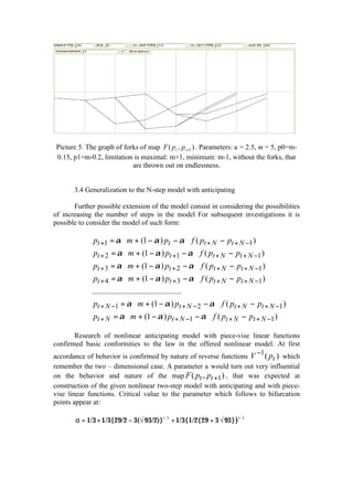
In the given work the offered two-step discrete model in time with anticipating
had been proposed and investigated. The main result of analysis of the maps is the
possibility of multy - valued transitions. In the paper all solutions of model are
explored. Some explanation of choice between these branches of solutions is also
proposed.
Remark that earlier a one – dimensional model with anticipation had been
used for money-economic processes [7, 8]. But the offered model has some principle
differences. The first is two- steps in transitions, that is passing on two steps ahead,
and second is that the function f(?) has a piece-vise linear character and belongs to the
class of neuron responses function which is usual for neural networks [9]. Piece -vise
linear character of function allowed making the thorough numerical - analytical
analysis. A new type of significant behavior had been found, when the region of
multy – valuedness in solutions is localized in space. At the end of work the example
of multy – step model is proposed is of which is more complicated by the dimension
of map. Because of presumable importance of results we also pose some discussion of
its possible applications to economical problems.

2. Model description

2.1 Prototype from economics

First of all we shortly describe the prototype model from the field of
economics. Here we pose the description of economical terms for illustration the
origin of prototype models. The nonlinear model of money - credit dynamics in
continuous time consists of equating of the price adjusting [6- 8]:

&
p = α [m − p − f (π )], (1)

&
where p - logarithm of price level, m - logarithm of amount (here it is foreseen to be
constant) of money, and p - the expected norm of inflation, that is:

&
π (t ) = Et [ p (t )], (2)

In accordance with equality (1), the norm of change of price at the market of
commodities relies on the surplus of demand for the real balances. The function f is
logarithm of demand for the real balances of money.
The discrete version of evolution equation of price (1) has such form:

pt +1 = α ⋅ m + (1 − α ) pt − αf (π t ,t +1 ), (3)

where now pt means logarithm of level of price in the moment of time of t. In
equality (3) the function of demand of money in the moment of time of t relies on the
norm of inflation of expected in a next period.

π t , t +1 = Et ( pt +1 − pt ), (4)

That to complete a definite model in (3) it is needed to take into account the
condition of passing ahead expectation. The hypothesis of passing ahead expectation
results in the one-dimensional map in a form for pt+1:

pt +1 = α ⋅ m + (1 − α ) pt − α ⋅ f ( pt +1 − pt ), (5)

Remark that the equation (5) had been derived as economical model but it is
(and other equations with anticipatory property) interesting mathematical object itself.

2.3 Two – step model of anticipatory element

Here we introduce a new nonlinear model which substantially extends the one
– dimensional equation (5). New features in proposed model are the next. The first is
two- steps nature (that is passing on two steps ahead). The second is that the function
f(?) has a piecewise - linear character, and looks like the transition function of neurons
in neuronets [9]. Remark that piecewise character of nonlinearity usually allows
developed mathematical investigations (see for example [10]).
We will write down the offered model as follows:

 pt +1 = α ⋅ m + (1 − α ) pt − α ⋅ f ( pt + 2 − pt +1 ) ( 6)

 pt + 2 = α ⋅ m + (1 − α ) pt +1 − α ⋅ f ( pt + 2 − pt +1 ) (7 )

The function f(x) depends on to the parameter a and has the following
expression:

 f ( x) = 0, x≤0

 f ( x) = α ⋅ x, x ∈ (0, 1α ] (8)
 f ( x) = 1,
 x > 1α

3 Model investigations
3.1 Inverse function representation

We will rewrite equation (7) thus, that pt + 2 were found for the right side of
equation.
( pt + 2 − pt +1 ) + α ⋅ f ( pt + 2 − pt +1 ) = α ⋅ m − α ⋅ pt +1 (9)

We will put this in right part of equation (6). Converting into a comfortable
form we will get the following equality:

( pt + 2 − pt +1 ) + α (1 − α ) f ( pt + 2 − pt +1 ) = α (1 − α )(m − pt ) (10)

We will enter the following function:

V ( x) = x + α (1 − α ) f ( x) (11)

Then we can write a next correlation

V ( pt + 2 − pt +1 ) = α (1 − α )(m − pt ) , from which we can receive

pt + 2 = pt +1 + V −1[α (1 − α )(m − pt )] ≡ F ( pt , pt +1 ) (12)

V −1 in equation (12) means the inverse function V, when V is invertible or
the proper function is definite by means one of inverting of function V, when V is not
uniquely invertible.
We will write down first derivative to the function V:

V ′( x) = 1 + α 2 f ′( x) − α 3 f ′( x) (13)

First derivative (13) to the function V at x < 0 that x > 1α has independent
from a value, according to properties of function f, equal to 1 accordant (11). We are
interested at the value of derivative function V at x ∈ (0,1/ α ] , so at exactly in this
interval the function of f matters dependency upon x accordant (8):

V ′( x) = 1 + α 2 − α 3 (14)

From equation (14) we have next results

α = 1/3 + 1/3{29/2 − 3(√ 93/2)}1/ 3 + 1/3{1/2{29 + 3 √ 93}}1/ 3

Approximate value is the next: a = 1.465...
2 3
Consequently subject to the condition 1 + α − α < 0 derivative to the
function V has the negative value, that can mean that the points of maximum appear,
and minimum of function V. And accordingly the ambiguousness of invertability of
function V appears which is represented on Picture 1.

Picture 1. The graph of function V, subjecting to the condition of ambiguous
invertability. Intervals (−∞,ν m ) and (VM , +∞) have one solution, interval (ν m , VM ) -
three solutions. Dotted line represents the reverse transformation of function V.

On Picture 1. we see a form of function V under a definite condition on a
parameter. We have the maximum of function V - VM in the point π 2 ( VM = V( π 2 ))
and minimum ν m in a point π 1 (ν m = V( π 1 )). There on graphic we see prototypes
?
V( π 2 ) and V( π 1 ) in other points π 2 and π1 accordingly. It is visible therefore, that
?

V −1 ( y ) has three separate points when vm < y <VM and one point otherwise. There
is a question how to represent a reverse function because the three special cases.
It is needed to remark that there is the fourth case, subject to the condition
1 + α 2 − α 3 = 0 for inverse function of V when there are not two points, but the
whole interval of points, which causes the endless quantity of possible variants of the
map F ( pt , pt +1 ) .
−1
Consequently, a function V determines the behavior of the map
F ( pt , pt +1 ) as follows. When V simply reversible, F ( pt , pt +1 ) is continuous, and non-
continuous, when V is not uniquely reversible.

3.2 Map F ( pt , pt +1 )

We will write out equation for the map F ( pt , pt +1 ) as follows:

F ( pt , pt +1 ) = pt +1 + V −1[α (1 − α )(m − pt )] (15)

The map F ( pt , pt +1 ) is continuous, when V reversible and is discontinuous
otherwise.
The fixed point:

V −1[α (1 − α )(m − pt )] = 0

 ⇒ α (1 − α )(m − pt ) = α (1 − α ) f (0)
V (0) = 0 + α (1 − α ) f (0) 


*
pt = m − f (0) = m (16)

As soon as F ( pt , pt +1 ) = pt +1 is achieved a condition

V −1[α (1 − α )(m − pt )] = 0 is executed, that is α (1 − α )(m − pt ) = V (0) , or
specifying the last expression α (1 − α )(m − pt ) = α (1 − α ) f (0) . When

F ( pt , pt +1 ) has the points of break, there it can be nonexisting of the fixed point,
however if exists, has a form in obedience to equality (16).
We will consider the cut of the map F ( pt , pt +1 ) =0. How visible with
Picture 2, right overhead part has the positive value, and the left lower part of cut
accordingly negative value. That is getting in a positive region, value of the map
F ( pt , pt +1 ) to be increased and increased to endlessness. Like there is the
reduction of value of map, at the hit in the negative region of values. If to set the
initial value from the region of ambiguousness close to the fixed point, on a next step,
the map will get a few values, one of which, will translate the map in a positive
region, the second value vice versa will translate the map in a negative region, that
will result in rejection of the state in endlessness, one in positive, second in negative.
And another solution will arise up, which will leave the state of map in the region of
ambiguousness. Thus there will be the permanent troop landing from the region of
ambiguousness in a plus and minus of endlessness. We can mark the region of
multivaluedness origin as the ‘boiling’ multy - valuedness. The term ‘boiling’ had
been introduced following visible analogy with boiling water tank when the
molecules of water leave tank through the free surface of water. Some solutions cross
the boundary of ‘rhomb’ and then tend to infinity. But some branches of solutions
stay within the ‘rhomb’ to undergo to further multiplication.

Picture 2. Cut of the map F ( pt , p t +1 ) = 0 at a parameter b>1.465.... Considered
equations (6) – (8) have three solutions in the rhomb on the plane (with marked three
vertexes m, 1* and 2*) and one solution in the rest of the plane.

Consequently, we are interested in the case, when the state of map is
constantly found in the region of ambiguousness. The most adjusted for such
investigation is computer calculation.

3.3 Behavior of the map F ( pt , pt +1 ) in state space

The software had been developed so that it is possible to visualize some
branches of the states of map, but only those, that are not thrown out to infinity, that
much facilitated understanding of processes, which take place in the region of

ambiguousness. Namely, on Picture 3 we can see two cycles of period 6, and the
quantity of cycles is multiplied in course of time, that is we can see a tendency to
phenomena which we may called „chaos”.

Picture 3. The graph of forks of the map F ( pt , p t +1 ) . Parameters: a = 3.2, m = 0, p0
=m-0.15, p1 =m-0.2, limitation is maximal: m+2, minimum: m-2, without the forks,
that are thrown out to infinity. The cycles are within the ‘rhomb’ with the multy -
valuedness above.

Picture 4. Map in state space. The sequence of values of ( pt , pt +1 ) is represented.
With reduction of parameter a the period of cycles diminishes. Diminishing
takes place until then, while a model can generate new cycles. As soon as a model
loses such power, a process goes out slowly. That it is possible to see on Picture 5
(cycles of period 4).

Picture 5. The graph of forks of map F ( pt , p t +1 ) . Parameters: a = 2.5, m = 5, p0=m-
0.15, p1=m-0.2, limitation is maximal: m+1, minimum: m-1, without the forks, that
are thrown out on endlessness.

3.4 Generalization to the N-step model with anticipating

Further possible extension of the model consist in considering the possibilities
of increasing the number of steps in the model For subsequent investigations it is
possible to consider the model of such form:

 pt +1 = α ⋅ m + (1 − α ) pt − α ⋅ f ( pt + N − pt + N −1 )
p
 t + 2 = α ⋅ m + (1 − α ) pt +1 − α ⋅ f ( pt + N − pt + N −1 )
 pt + 3 = α ⋅ m + (1 − α ) pt + 2 − α ⋅ f ( pt + N − pt + N −1 )

 pt + 4 = α ⋅ m + (1 − α ) pt + 3 − α ⋅ f ( pt + N − pt + N −1 )
...........................................

 pt + N −1 = α ⋅ m + (1 − α ) pt + N − 2 − α ⋅ f ( pt + N − pt + N −1 )

 pt + N = α ⋅ m + (1 − α ) pt + N −1 − α ⋅ f ( pt + N − pt + N −1 )
Research of nonlinear anticipating model with piece-vise linear functions
confirmed basic conformities to the law in the offered nonlinear model. At first
−1
accordance of behavior is confirmed by nature of reverse functions V ( pt ) which
remember the two – dimensional case. A parameter a would turn out very influential
on the behavior and nature of the map F ( pt , pt +1 ) , that was expected at
construction of the given nonlinear two-step model with anticipating and with piece-
vise linear functions. Critical value to the parameter which follows to bifurcation
points appear at:

α = 1/3 + 1/3{29/2 − 3(√ 93/2)}1/ 3 + 1/3{1/2{29 + 3 √ 93}}1/ 3

It is needed to remark that there is the fourth case, subject to the condition at
the inverse to function V when there are not two points, but a whole interval of points,
which causes the infinite number of possible variants of the map F ( pt , pt +1 ) .
−1
A function V determines the conduct of the map F ( pt , pt +1 ) as follows.
When V simply reversible, F ( pt , pt +1 ) is continuous, and otherwise when a
function V is not uniquely reversible. But just in the preliminary investigations some
new possibilities had been found. For examples for some parameters value we had
found the possibilities of increasing the number of branches during time increasing.

Summary

So in proposed paper we have considered some examples of anticipatory
models – namely discrete – time models of single element with two – step anticipation
in time. Chosen form of nonlinearity (piecewise - linear) allowed considering in
details the dynamical behavior of solutions, branching of solutions and possible ways
for some type of complex behavior related with possible multy - valuedness. These
results are interesting and new per se. But it may be supposed that such type of
models may constitute one of the interesting fields of mathematical investigations of
anticipatory system. Just many – step in time equations from Paragraph 3.4 are
interesting objects. But much more interesting may be investigations of coupled
systems of anticipated elements. One of the most important classes of such systems
constitutes the multy – valued neuronal networks [5]. In case of the artificial neuronal
networks usually some of the research problems are the architecture of networks,
leading principles and investigations of their behavior. Remark that now we make
some investigations on such networks.
Other wide new class of research problem is the investigation of self –
organization processes in the anticipating media, in particular in discrete chains,
lattices, networks from anticipating elements. In such case the main problems are self
– organization, emergent structures including dissipative, bifurcations,
synchronization and chaotic behavior [11]. As it is seen from previous paragraphs
such problems take new forms of presumable possible multy – valuedness in
anticipatory systems. For example just definition of ‘chaos’ in such case should be
reconsidered. Remark that such problems are new for recent theory. But currently
already understanding of such phenomena possibilities may help in investigation and
managing real systems. Especially important may be applications to social,
economical etc. systems. Some outlines of possibilities were discussed in [3, 4]. The
realizations of such research programs are the goals for further investigations. Here
we pose only some discussion on possible applications of proposed models in
economics.
Recently the ideas of anticipatory nature of ‘homo economicus’ (participant of
economical relation) and organizations explicitly (but sometimes only verbally)
penetrate into the community of theoretic and practitioners in economy. Currently
some explicit investigations of macro economical models with anticipation had been
proposed [12, 13]. But these investigations are concentrated mainly on the stability
problems.
Described in present paper results extended to the new society models open
the new possibilities for exploring economical behavior. The key is possible multy –
valuedness in such systems and new understanding on decision – making role. As one

of possible topics for considerations we may foresee the investigation if uncertainty in
such systems. Now one of the leading ideas is the the uncertainty in economical
systems origins from dynamical chaos in it [14]. But as it follows from our
investigations anticipation and multy – valuedness also may serve as the source of
uncertainty in economical systems. Then presumable new tools for managing such
uncertainty may follows from mathematical modeling of anticipatory economical
systems.
Thus in proposed paper we have discussed strict results on some mathematical
models with anticipation and possible related issues, especially for economical
systems. We hope that further investigation will follow to next new and interesting
results.

References

1. Rosen R. Anticipatory Systems. Pergamon Press. 1985.
2. Dubois D. Introduction to computing Anticipatory Systems.. International Journal of
Computational Anticipatory .Systems, 1998. Vol. 2. pp. 3-14.
3. Makarenko A. Anticipating in modeling of large social systems - neuronets with internal structure
and multivaluedness. International .Journal of .Computational Anticipatory Systems, Vol. 13., pp.
77 - 92. 2002.
4. Makarenko A. Anticipatory agents, scenarios approach in decision- making and some quantum –
mechanical analogies. International Journal of Computational Anticipatory Systems, Vol. 15.,
pp.217 - 225. 2004.
5. Makarenko A. Multi- valued neuronets and their mathematical investigations
problem // Abstract books5 th Int.Math. School: Liapunov functions method and
applications. Simpheropol, Ukraine, Creamia, Tavria University, 2000. p. 116.
6. Sargent T.J, Wallice B. Stability of money and growth models with perfect
foresees. Econometrica 1973, vol. 41. pp. 1043–1048.
7. Agliari A., Chiarella C., Gardini L. A stability analysis of the perfect foresight map
in nonlinear models of monetary dynamics, Chaos, Solitons and Fractals, vol. 21
2004. pp.371 -386.
8. Mira C., Gardini L., Barugola A., Cathala J.C., Chaotic dynamics in two-
dimensional noninvertible maps. Singapore: World Scientific, 1996.
9. Haykin S., Neural Networks: Comprehensive Foundations. MacMillan: N.Y., 1994.
10. Maistrenko Yu., Kapitaniak T., Szuminski P. Locally and globally basin in
two coupled piecewise – linear maps. Phys.Rev.E , vol.E56, pp. 6393 – 6399,
1997.
11. Nicolis G., Prigogine I. Self – organization in nonequilibrium systems.
N.Y., John Wiley & Sons, 1977.
12. Dubois D., Holmberg S. Modeling and simulation of management systems
with retardation and anticipation. Abstract book of Int. Conf. CASYS’05,
August 2005, Liege, p.5/5
13. Leydersdirf L. Hyper – incursion and the globalization of the knowledge –
based economy. Abstract book of Int. Conf. CASYS’05, August 2005, Liege,
p.8/8.
14. Dendrinos D. Chaos: challenges from and to socio- spatial form and policy.
Discrete dynamics in nature and society. Vol.1, pp.9- 15, 1997.

Some Two-Steps Discrete-Time Anticipatory Models with ‘Boiling’ Multivaluedness

More Related Content

What's hot

Viewers also liked

Similar to Some Two-Steps Discrete-Time Anticipatory Models with ‘Boiling’ Multivaluedness

More from SSA KPI

Recently uploaded

Some Two-Steps Discrete-Time Anticipatory Models with ‘Boiling’ Multivaluedness