Download to read offline
![Solve Polynomial and transcendental Equations
with use Generalized Theorem (Method Lagrange)
N.Mantzakouras
e-mail: nikmatza@gmail.com
Athens – Greece
Abstract
While all the approximate methods mentioned or others that exist, give some specific solu-
tions to the generalized transcendental equations or even polynomial, cannot resolve them com-
pletely.”What we ask when we solve a generalized transcendental equation or polynomials, is to
find the total number of roots and not separate sets of roots in some random or specified inter-
vals. Mainly because too many categories of transcendental equations have an infinite number of
solutions in the complex set.” There are some particular equations (with Logarithmic functions,
Trigonometric functions, power function, or any special Functions) that solve particular prob-
lems in Physics, and mostly need the generalized solution. Now coming the this theory, using
the generalized theorem and the Lagrange method, which deals with hypergeometric functions or
interlocking with others functions, to gives a very satisfactory answer by use inverses functions
and give solutions to all this complex problem”.
The great logical innovation of the Generalized Theorem is that is gives us the philosophy to
work out the knowledge that the plurality of roots of any equation depends on the sub-fields of
the functional terms of the equation they produce. Thus the final field of roots of the equation
will be the union of these sub-fields.
keywords: Transcendental equations, solution, Hypergeometric functions,
field-subfield of roots, Polynomial, famus equations.
Part I.
I.1.Indroduction
According to the logic of the Generalized Theory of the Existence of Roots that we need and with which
we will deal after, and we before to prove, we will mention some elements more specifically for a random
general transcendental equation whish apply:
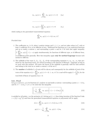
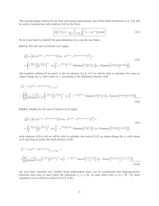
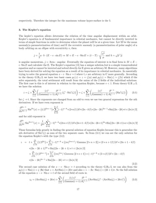
f(z) =
n
X
i=1
mi · pi(z) + t = 0 (1.1)
with pi(z) functions of z in C, Primary simple transcendental equations, will be in effect the two initial
types (1.2, 1.3) with name LMfunction:
ϕk(w) =
n
X
i=1,i6=k
(mi/mk) · pi p−1
k (w)
(1.2)
∀i, k ≥ 1, i 6= k, {i, k ≤ n}
1
arXiv:2107.14595v1
[math.GM]
21
Jul
2021](https://image.slidesharecdn.com/solveequationse-220223205749/85/Solve-Equations-2-320.jpg)
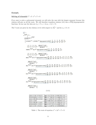
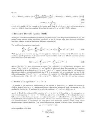
![for polynomials with n terms or transcendental equations in order to achieve a better and more efficient
solution. The general equation now of Lagrange is:
f(ζ) = f(w)w→−t/mk
+
∞
X
n=1
(−1)
n
n!
dn−1
dwn−1
[(f(w))0
{ϕ(w)}n
]w→−t/mk
(1.3)
All cases of equations start from the original function (1.4), with a very important relation:
pk(z) = −
t
mk
, k ≥ 1 ∧ k ≤ n (1.4)
If we assume now that it is apply from initial one pκ(z) = w, in Domain of, then if we apply the corresponding
transformation of the original equation (1.1), will be have,
ζ = z = p−1
κ (w) ⇔ pk(z) = w (1.5)
where after the substitution in the basic relation (1.3) and because here apply the well-known theorem
(Burman-Lagrange) we can calculate the any root of the equation (1.1).
But this previous standing theory is not enough to solving a random equation that will be (transcendental in
general) because it does not explain what is the number of roots and what it depends on. We will therefore
need a generalized theorem that gives us more information about the structure of an equation. We will
call this theorem the ”Generalized existence theorem and global finding of the roots of a random
transcendental or polynomial equation in the complex plane C or more simple Generalised
theorem of roots an equation”
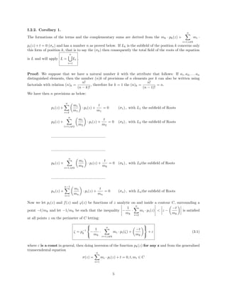
I.2. Generalized roots theorem of an equation.(G.RT.L)
For each random transcendental or polynomial equation, of the form
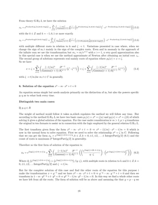
σ(z) =
n
X
i=1
mi · pi(z) + t = 0, t, mi ∈ C (2.1)
it has as its root set the union of the individual fields of the roots, which are generated by the following
functions (of number n) which are at the same time and the terms of
m1 · p1(z) +
n
X
i=2
mi · pi(z) + t = 0 (σ1)
m2 · p2(z) +
n
X
i=1,j6=2
mi · pi(z) + t = 0 (σ2)
.....................................................
.....................................................
2](https://image.slidesharecdn.com/solveequationse-220223205749/85/Solve-Equations-3-320.jpg)
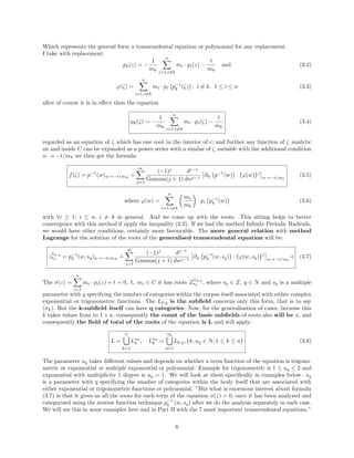
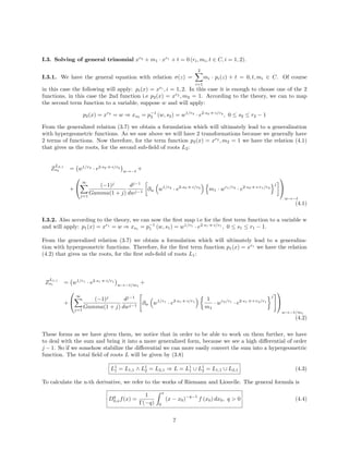

The document presents a research proposal focused on solving polynomial and transcendental equations using a generalized theorem based on Lagrange's method. It emphasizes the need for finding all roots rather than specific subsets, introducing concepts related to hypergeometric functions and the philosophy of root plurality based on functional terms. The generalized existence theorem proposed seeks to provide a comprehensive framework for understanding and solving these complex equations.