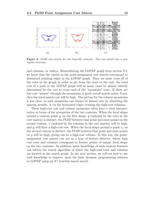
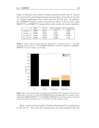
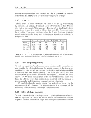
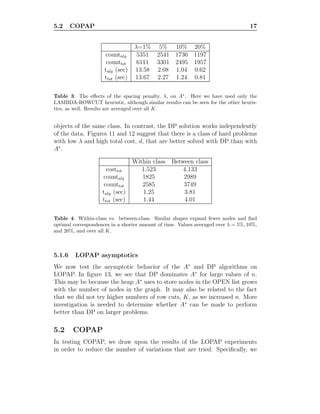
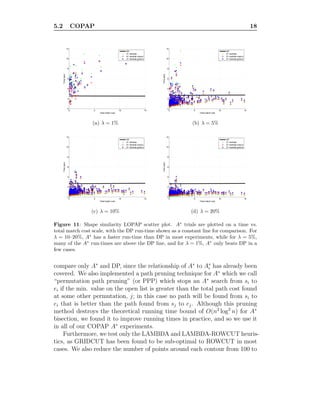
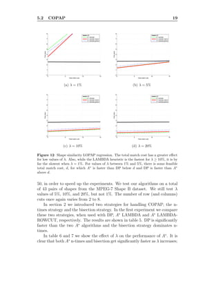
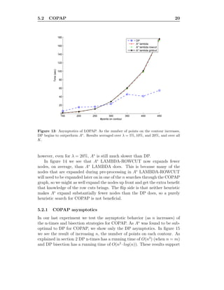
This document summarizes a paper that presents new algorithms for solving the cyclic order-preserving assignment problem (COPAP) and related sub-problem, the linear order-preserving assignment problem (LOPAP). It introduces a new point-assignment cost function called the Procrustean local shape distance (PLSD) and explores heuristics for using the A* search algorithm to more efficiently solve COPAP and LOPAP. Experimental results on the MPEG-7 shape dataset are presented and recommendations are made for solving COPAP/LOPAP in practice.
![1 Introduction and motivation 1
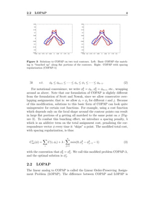
Figure 1: Order-preserving matching (left) vs. Non-order-preserving matching (right),
from the inner shape to the outer shape.
Abstract
In this paper, we present a new point-assignment cost function–called
the Procrustean local shape distance (PLSD)–for use with the cyclic order-
preserving assignment problem (COPAP). We present a variation of COPAP
called COPAP-λ in order to give higher cost to matchings which “bunch”
points together in the assignment. We then explore three novel heuristics for
use with the A∗ search algorithm in order to solve COPAP and its related sub-
problem, LOPAP, more efficiently. We compare the performance of these new
A∗ algorithms to the dynamic programming solutions given in the existing
literature on the MPEG-7 shape B data set.
1 Introduction and motivation
Most shape modeling and recognition algorithms rely on being able to solve
a correspondence problem between parts of two or more objects. In 2-D, a
shape is often represented as a closed contour [3, 7, 14, 16, 25]. Some methods
use continuous representations of shape contours, matching curve segments
on one contour to those on another [23], or matching the control points of
two active contours [9]. Others use the skeleton of a contour to represent
the shape of an object [24, 26]. For these methods, skeletal tree branches
must be matched to each other, and a tree edit distance is often employed
to determine the similarity between shapes.
In this paper, we represent the shape of an object by a densely-sampled,
ordered set of discrete points around its contour, where one must find an
optimal assignment of the points on one contour to the points on another
contour. Within this framework, a large body of literature exists on shape
recognition and retrieval [7, 10, 16], as well as on statistical shape modeling [5,
6, 12, 13, 27]. In each case one must solve the correspondence problem in
order to proceed.
In order to find correspondences between the points of two contours,
one typically gives a cost function, C(i, j), for assigning point i on the first](https://image.slidesharecdn.com/f8c61b26-3292-4938-a439-6ebd08372f53-160708130118/85/10-1-1-630-8055-2-320.jpg)
![1.1 Point Assignment Cost Functions 2
−0.25 −0.2 −0.15 −0.1 −0.05 0 0.05 0.1 0.15 0.2
−0.25
−0.2
−0.15
−0.1
−0.05
0
0.05
0.1
0.15
0.2
0.25
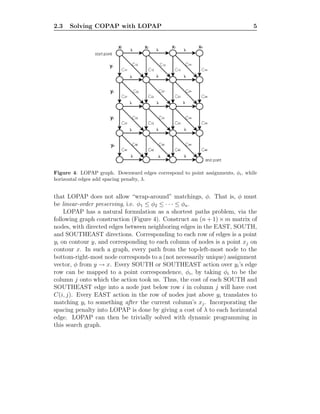
Figure 2: Tool articulation. Euclidean distance cost function is sensitive to articulation
and concavities, as well as to the initial alignment (in this case by ICP).
contour to point j on the second contour, and these costs are usually as-
sumed to all be independent. In addition, we may have constraints on the
matching; for example, we may require a one-to-one matching or an order-
preserving matching (Figure 1). Scott and Nowak [22] define the Cyclic
Order-Preserving Assignment Problem (COPAP) as the problem of finding
an optimal matching such that the assignment of corresponding points pre-
serves the cyclic ordering inherited from the contours. Alternatively, if we
don’t require the assignment to preserve contour ordering, yet we do de-
sire a one-to-one matching, the problem may be formulated as a bipartite
matching [1] or as a relaxation labeling [21].
1.1 Point Assignment Cost Functions
One recent approach which has had some success using the point-assignment
cost framework is that of shape contexts [1]. The shape context of a point
captures the relative positions of other points on the contour in a log-polar
histogram. The point assignment cost is determined by a χ2
distance between
corresponding shape context histograms.
Another option is to simply align the two shapes as closely as possible, e.g.
using a Hausdorff distance [8] or Iterated Closest Point (ICP) [2], and then to
compute the cost function between two points as the Euclidean distance from
one point to the other. Unfortunately, this method can give poor results when
the contours have large concavities on them, or in the presence of articulation
(e.g. the opening and closing of a tool–figure 2). It is also extremely sensitive
to the initial alignment, so such methods should only be used when it is
known, a priori, that the two shapes will be very similar.](https://image.slidesharecdn.com/f8c61b26-3292-4938-a439-6ebd08372f53-160708130118/85/10-1-1-630-8055-3-320.jpg)
![1.2 Overview 3
A third method, which we will use in this paper, is to use local, rather
than global shape information at each point, comparing the shapes of neigh-
borhoods around the two points in order to determine the point assignment
cost. To do this, we will draw on the body of work known as Shape Theory,
pioneered by D.G. Kendall [12] and others [5, 6] in order to provide a mathe-
matical foundation for comparing the shapes of ordered sets of points. One of
the central results of shape theory is the formulation of the Procrustes met-
ric as a distance metric in shape space, which is invariant under translation,
scaling, and rotation, and is thus very desirable for comparing shapes. We
will use this Procrustes shape metric to compute the shape distance between
two point neighborhoods, and will then take the point-assignment cost as the
minimum neighborhood shape distance over varying neighborhood sizes.
1.2 Overview
The paper will proceed as follows: First we will describe the Cyclic Order-
Preserving Assignment Problem (COPAP), as well as the related Linear
Order-Preserving Assignment Problem (LOPAP). We will then present al-
gorithms to solve COPAP and LOPAP, along with their theoretical bounds.
Next, we will discuss how the choice of point-assignment cost function effects
the structure of the problem, and present several heuristic search algorithms
which attempt to take advantage of this structure. Finally, experimental
results will be shown using the MPEG-7 shape database [15, 4], and we will
conclude with some recommendations for solving LOPAP/COPAP in prac-
tice.
2 Problem formulation
2.1 COPAP
We wish to match the points of one closed contour, y1, ..., yn to the points
on another closed contour, x1, ..., xm . (Here we use · to indicate that the
points are ordered, and thus form a vector.) Let φ denote a correspondence
vector, where φi is the index of x to which yi corresponds; that is: yi →
xφi
. Then, given a point-assignment cost function, C(i, φi), the basic Cyclic
Order-Preserving Assignment Problem (COPAP) is:
φ∗
= arg min
φ
i
C(i, φi) s.t. φ is cyclic order-preserving (1)
where φ is cyclic order-preserving if and only if](https://image.slidesharecdn.com/f8c61b26-3292-4938-a439-6ebd08372f53-160708130118/85/10-1-1-630-8055-4-320.jpg)
![2.4 A Bisection Strategy for COPAP 7
s1
s2
s3
s4
e1
e2
e3
e4
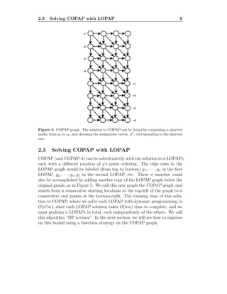
Figure 6: COPAP bisection strategy. Each shortest path from si to ei is constrained to
lie between the shortest paths below and above it.
2.4 A Bisection Strategy for COPAP
Consider the state of the “DP n-times” algorithm after finding a shortest path
from si to ei, but before finding the shortest path from si+1 to ei+1 (Figure 6).
The shortest path from si+1 to ei+1 must lie below the shortest path from
si to ei, since any path from si+1 to ei+1 which crosses over the previous
shortest path would have been better off to have followed the shortest path
between the intersection points rather than taking the detour above it. The
same argument applies if we have already computed paths below si+1 → ei+1,
so that we can constrain our search space from above and below, depending
on the order in which paths are found in the COPAP graph.
From [18], we see that the best order in which to compute the shortest
paths is a bisection ordering, starting with sn/2 → en/2 at the first level,
then sn/4 → en/4 and s3n/4 → e3n/4 at the second level, and so on. There
are O(log n) levels in total, and at each level we perform a series of disjoint
bounded searches, with a total of O(nm) work being done in the DPs at each
level. Thus, the total running time of this bisection algorithm, which we call
“DP bisection”, is O(nm log n).
3 Point Assignment Cost
We use a novel point assignment cost function, which we call the Procrustean
Local Shape Distance (PLSD). A formal justification of this cost function is](https://image.slidesharecdn.com/f8c61b26-3292-4938-a439-6ebd08372f53-160708130118/85/10-1-1-630-8055-8-320.jpg)
![3.1 Procrustean Local Shape Distance 8
beyond the scope of this paper–for now it suffices to say that PLSD belongs
to a class of point assignment cost functions which consider local, rather
than global shape information, and which use the geometry of the contour
itself, rather than using derived statistics such as curvature or medial axis
skeletons, in order to compute a similarity measure between the local shapes
of contour points. PLSD is similar in nature to Belongie’s shape contexts [1],
in that both methods directly use the observed geometry of the contour in
order to compute the shape signature of a point. However, shape contexts
consider the relative global shape with respect to each point, while the PLSD
captures only local shape information.
Another attribute of our approach is that the PLSD is a multi-resolution
similarity measure–it compares local shapes of varying sizes in order to de-
termine the overall match quality. The only other shape model we are
aware of to use such a multi-resolution technique is the curvature scale space
model [19], where contours are convolved with Gaussian kernels of varying
sizes. Also similar to our method is the SIFT feature representation [17],
which also use multi-resolution information to compare features, although
SIFT features are computed on images, while the PLSD applies to contours.
3.1 Procrustean Local Shape Distance
The Procrustes distance, dP , between two point vectors, x and y, is a metric
on Kendall’s shape space [13] which is invariant to rotation, translation, and
scaling of the point vectors x and y. In related work [7], we use the Procrustes
distance to compute distributions over shapes in the same shape class in order
to achieve robust shape classification and completion of occluded parts of
contours. Given its utility for such shape inference tasks, it seems natural to
attempt to apply the same Procrustean shape metric to the correspondence
problem.
Given a point xi on contour x, we define the local neighborhood of size k
(for k odd) as:
ηk(xi) = xi−(k−1)/2, ..., xi, ..., xi+(k−1)/2 (4)
The Procrustean Local Shape Distance, dP LS, between two points, xi and
yj is the minimum Procrustean shape distance over varying neighborhood
sizes, k:
dP LS(xi, yj) = min
k
dP [ηk(xi), ηk(yj)] (5)](https://image.slidesharecdn.com/f8c61b26-3292-4938-a439-6ebd08372f53-160708130118/85/10-1-1-630-8055-9-320.jpg)
![4 Heuristic Search 11
4 Heuristic Search
While the basic DP solution to COPAP yields a good asymptotic running
time–O(nm log n)–using the bisection strategy of section 2.4, the story for
LOPAP is not nearly as good. Although it is impossible to improve upon
DP’s worst-case asymptotic running time of Θ(nm), the DP solution expands
all (n + 1) × m states in the LOPAP graph, while many of these states may
never need to be considered in a heuristic search.
In this section, we present several different cost-to-goal heuristic functions
for use with the A* search algorithm [20]. The first of these we call the
LAMBDA heuristic, as it uses the spacing penalty, λ, to determine a lower
bound on the cost-to-goal. The second is the ROWCUT heuristic, which uses
prior knowledge of the high-cost rows in the point-assignment cost matrix
in order to lower bound the cost-to-goal, and the third is the GRIDCUT
heuristic, which uses prior knowledge of both the high cost rows and the
high cost columns. In practice, we may combine these heuristics, at any
node taking the h-function with maximum value (since they are all lower
bounds), or for heuristics which are independent (such as LAMBDA and
ROWCUT), we may add their h-values together to create a new heuristic.
4.1 The LAMBDA heuristic
Each horizontal edge in the LOPAP graph has a cost of λ. In addition, we
may never move up or to the left in the graph. Thus, if we are currently
standing at a node in the bottom-left portion of the LOPAP graph, we must
pay some spacing penalty in order to walk the rest of the way to the goal.
We can lower bound this spacing penalty by λ times the horizontal distance
from the diagonal; that is:
hλ(i, j) = [max(0, (jg − j) − (ig − i))] · λ (6)
where (i, j) is the current position in the graph (row, column), and (ig, jg)
is the position of the goal–for LOPAP, (n + 1, m).
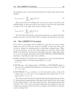
4.2 The ROWCUT heuristic
In order to reach the goal from any node in the LOPAP graph, we must
cross over every row of edges between the current node and the goal. In
particular, we must cross over all of the high-cost, or mountain rows between
the two nodes. Thus, given that the cost matrix has been computed for K
high-cost rows, r1, ..., rK, we can lower bound the cost-to-goal as the sum of](https://image.slidesharecdn.com/f8c61b26-3292-4938-a439-6ebd08372f53-160708130118/85/10-1-1-630-8055-12-320.jpg)
![5 Experimental Results 13
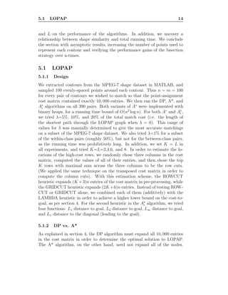
5 Experimental Results
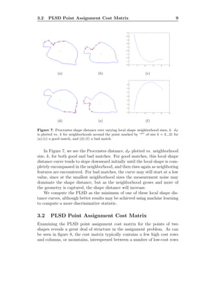
Figure 9: Some of the shapes from the MPEG-7 Shape B dataset used in the experiments.
We tested the COPAP and LOPAP algorithms discussed above on a total
of 390 randomly drawn pairs of shapes from the MPEG-7 Shape B dataset
(Figure 9). 360 pairs were drawn from the same class, and 60 from different
classes. We designed the sampling to be imbalanced in this way because in
most practical applications, the contour-based correspondence algorithms we
have considered only give meaningful results when run on pairs of shapes that
are similar to each other; more complex, part-based methods should be used
to compare shapes that are very different. All algorithms were implemented
in a mix of MATLAB and C code, with the heavy pointer-arithmetic and
data structure code being written in C, and everything else in MATLAB.
In particular, this means that the PLSD point-assignment cost function was
implemented in MATLAB, and thus made up a very significant portion of the
total running time of our algorithms. This is not an unreasonable feature,
however, since many point-assignment cost functions are even more compu-
tationally expensive than the PLSD, and we would like our analysis to apply
to those methods as well.
The experiments will be presented in two parts. First, we test LOPAP,
comparing the dynamic programming solution in section 2.2 to the A∗
algo-
rithms in section 4. In addition, we compare A∗
, which yields optimal solu-
tions, to A∗
ǫ [20], an approximation algorithm, with varying second heuristic
function, h2
1
. In the second part of this section, we test COPAP, compar-
ing the “DP n-times” and “DP bisection” algorithms from sections 2.3–2.4
to “A∗
n-times” and “A∗
bisection”, the equivalent algorithms where each
LOPAP is solved with A∗
instead of dynamic programming.
We also investigate the effects of both model and algorithmic parameters–
namely the spacing penalty, λ, and the number of row and column cuts, K
1
The second heuristic function of A∗
ǫ gives the expansion order of all nodes within ǫ%
of the current minimum f-value.](https://image.slidesharecdn.com/f8c61b26-3292-4938-a439-6ebd08372f53-160708130118/85/10-1-1-630-8055-14-320.jpg)
![REFERENCES 24
−0.25 −0.2 −0.15 −0.1 −0.05 0 0.05 0.1 0.15 0.2
−0.25
−0.2
−0.15
−0.1
−0.05
0
0.05
0.1
0.15
0.2
0.25
−0.25 −0.2 −0.15 −0.1 −0.05 0 0.05 0.1 0.15 0.2
−0.25
−0.2
−0.15
−0.1
−0.05
0
0.05
0.1
0.15
0.2
0.25
−0.25 −0.2 −0.15 −0.1 −0.05 0 0.05 0.1 0.15 0.2
−0.25
−0.2
−0.15
−0.1
−0.05
0
0.05
0.1
0.15
0.2
0.25
−0.25 −0.2 −0.15 −0.1 −0.05 0 0.05 0.1 0.15 0.2 0.25
−0.25
−0.2
−0.15
−0.1
−0.05
0
0.05
0.1
0.15
0.2
0.25
Figure 16: Optimal solutions to COPAP-λ with the PLSD point-assignment cost func-
tion.
References
[1] Serge Belongie, Jitendra Malik, and Jan Puzicha. Shape matching and
object recognition using shape contexts. IEEE Trans. Pattern Analysis
and Machine Intelligence, 24(24):509–522, April 2002.
[2] P.J. Besl and N.D. McKay. A method for registration of 3-d shapes.
IEEE Transactions on Pattern Analysis and Machine Intelligence,
14(2):239–256, 1992.
[3] A. Blake and M. Isard. Active Contours. Springer-Verlag, 1998.
[4] Miroslaw Bober. Mpeg-7 visual shape descriptors. IEEE Trans. on
Circuits and Systems for Video Technology, 11(6), June 2001.
[5] F.L. Bookstein. A statistical method for biological shape comparisons.
Theoretical Biology, 107:475–520, 1984.
[6] I. Dryden and K. Mardia. Statistical Shape Analysis. John Wiley and
Sons, 1998.
[7] Jared Glover, Daniela Rus, Nicholas Roy, and Geoff Gordon. Robust
models of object geometry. In Proceedings of the IROS Workshop on
From Sensors to Human Spatial Concepts, Beijing, China, 2006.](https://image.slidesharecdn.com/f8c61b26-3292-4938-a439-6ebd08372f53-160708130118/85/10-1-1-630-8055-25-320.jpg)
![REFERENCES 25
[8] D.P. Huttenlocher, G.A. Klanderman, and W.A. Rucklidge. Comparing
images using the hausdorff distance. IEEE Transactions on Pattern
Analysis and Machine Intelligence, 15(9):850–863, 1993.
[9] M. Isard and A. Blake. Contour tracking by stochastic propagation of
conditional density. In European Conf. Computer Vision, pages 343–356,
1996.
[10] V. Jain and Robust 2D shape Correspondence using Geodesic
Shape Context H. Zhang. Robust 2d shape correspondence using
geodesic shape context. Pacific Graphics, pages 121–124, May 2005.
[11] D.G. Kendall. The diffusion of shape. Advances in Applied Probability,
9:428–430, 1977.
[12] D.G. Kendall. Shape manifolds, procrustean metrics, and complex pro-
jective spaces. Bull. London Math Soc., 16:81–121, 1984.
[13] D.G. Kendall, D. Barden, T.K. Carne, and H. Le. Shape and Shape
Theory. John Wiley and Sons, 1999.
[14] L. J. Latecki and R. Lak¨amper. Contour-based shape similarity. In
Proc. of Int. Conf. on Visual Information Systems, volume LNCS 1614,
pages 617–624, June 1999.
[15] Longin Jan Latecki, Rolf Lak¨amper, and Ulrich Eckhardt. Shape de-
scriptors for non-rigid shapes with a single closed contour. In IEEE Conf.
on Computer Vision and Pattern Recognition (CVPR), pages 424–429,
2000.
[16] Haibin Ling and David W. Jacobs. Using the inner-distance for clas-
sification of articulated shapes. IEEE Computer Vision and Pattern
Recognition, 2:719–726, June 2005.
[17] David G. Lowe. Object recognition from local scale-invariant features.
In Proc. of the International Conference on Computer Vision ICCV,
pages 1150–1157, 1999.
[18] Maurice Maes. On a cyclic string-to-string correction problem. Inf.
Process. Lett., 35(2):73–78, 1990.
[19] F. Mokhtarian and A. K. Mackworth. A theory of multiscale curvature-
based shape representation for planar curves. In IEEE Trans. Pattern
Analysis and Machine Intelligence, volume 14, 1992.](https://image.slidesharecdn.com/f8c61b26-3292-4938-a439-6ebd08372f53-160708130118/85/10-1-1-630-8055-26-320.jpg)
![REFERENCES 26
[20] Judea Pearl. Heuristics: Intelligent Search Strategies for Computer
Problem Solving. Addison-Wesley, Reading, MA, 1984.
[21] S. Ranade and A. Rosenfeld. Point pattern matching by relaxation.
Pattern Recognition, 12:269–275, 1980.
[22] C. Scott and R. Nowak. Robust contour matching via the order pre-
serving assignment problem. IEEE Transactions on Image Processing,
15(7):1831–1838, July 2006.
[23] Thomas Sebastian, Philip Klein, and Benjamin Kimia. On aligning
curves. PAMI, 25(1):116–125, January 2003.
[24] Thomas Sebastian, Philip Klein, and Benjamin Kimia. Recognition of
shapes by editing their shock graphs. volume 26, 2004.
[25] Thomas B. Sebastian and Benjamin B. Kimia. Curves vs skeletons in
object recognition. Signal Processing, 85(2):247–263, February 2005.
[26] Kaleem Siddiqi, Ali Shokoufandeh, Sven J. Dickinson, and Steven W.
Zucker. Shock graphs and shape matching. In ICCV, pages 222–229,
1998.
[27] C. G. Small. The statistical theory of shape. Springer, 1996.
[28] Remco C. Veltkamp. Shape matching: Similarity measures and algo-
rithms. Technical Report UU-CS-2001-03, Utrecht University, 2001.
[29] Yefeng Zheng and David Doermann. Robust point matching for nonrigid
shapes by preserving local neighborhood structures. IEEE Transactions
on Pattern Analysis and Machine Intelligence, 28(4), April 2006.](https://image.slidesharecdn.com/f8c61b26-3292-4938-a439-6ebd08372f53-160708130118/85/10-1-1-630-8055-27-320.jpg)