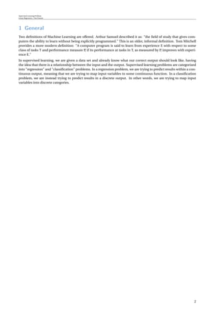
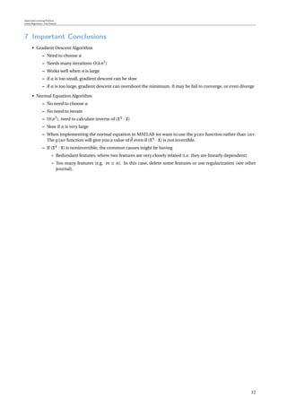
1. The document describes supervised learning problems, specifically linear regression with one feature. It defines key concepts like the hypothesis function, cost function, and gradient descent algorithm. 2. A data set with one input feature and one output is defined. The goal is to learn a linear function that maps the input to the output to best fit the training data. 3. The hypothesis function is defined as h(x) = θ0 + θ1x, where θ0 and θ1 are parameters to be estimated. Gradient descent is used to minimize the cost function and find the optimal θ values.

1. MACHINE LEARNING COLLECTION
THEORIE
Supervised Learning Problem
Linear Regression / One Feature
Marco Moldenhauer
May 31, 2017

2. Supervised Learning Problem
Linear Regression / One Feature
1 General
Two definitions of Machine Learning are offered. Arthur Samuel described it as: "the field of study that gives com-
puters the ability to learn without being explicitly programmed." This is an older, informal definition. Tom Mitchell
provides a more modern definition: "A computer program is said to learn from experience E with respect to some
class of tasks T and performance measure P, if its performance at tasks in T, as measured by P, improves with experi-
ence E."
In supervised learning, we are given a data set and already know what our correct output should look like, having
the idea that there is a relationship between the input and the output. Supervised learning problems are categorized
into "regression" and "classification" problems. In a regression problem, we are trying to predict results within a con-
tinuous output, meaning that we are trying to map input variables to some continuous function. In a classification
problem, we are instead trying to predict results in a discrete output. In other words, we are trying to map input
variables into discrete categories.
2

3. Supervised Learning Problem
Linear Regression / One Feature
2 Data Set
We define a input set Ω with one bias element x0 and one feature element x1 and a output set Υ with one output
element y1.
Ω = {x0;x1} (2.1)
Υ = {y1} (2.2)
An arbitrary element u ∈ Ω and v ∈ Υ are vectoriezed by m rows.
x0 =


















x(1)
0
x(2)
0
x(3)
0
...
x(i)
0
...
x(m)
0


















=


















1
1
1
...
1
...
1


















(2.3)
x1 =


















x(1)
1
x(2)
1
x(3)
1
...
x(i)
1
...
x(m)
1


















(2.4)
y1 =


















y(1)
1
y(2)
1
y(3)
1
...
y(i)
1
...
y(m)
1


















(2.5)
We define a set Π with m tuple called training set.
Π = {(1,x(1)
1 , y(1)
1 ); (1,x(2)
1 , y(2)
1 ); (1,x(3)
1 , y(3)
1 ); ... ;(1,x(i)
1 , y(i)
1 ); ... ;(1,x(m)
1 , y(m)
1 )} (2.6)
3

4. Supervised Learning Problem
Linear Regression / One Feature
For a better intuition of the training set we can write it in a table called training table. Every row means one training
example. In total we have m training examples.
1 x(1)
1 y(1)
1
1 x(2)
1 y(2)
1
1 x(3)
1 y(3)
1
...
...
...
1 x(i)
1 y(i)
1
...
...
...
1 x(m)
1 y(m)
1
Table 2.1 Training table
We define the discrete training function t(x(i)
1 ):
t : {x(1)
1 ;x(2)
1 ;x(3)
1 ;... ;x(i)
1 ;... ;x(m)
1 } → {y(1)
1 ; y(2)
1 ; y(3)
1 ;... ; y(i)
1 ;... ; y(m)
1 } (2.7)
x(i)
1 → y(i)
1
We define a matrix T called training matrix. We also define the input matrix X and the output matrix Y.
T =


















1 x(1)
1 y(1)
1
1 x(2)
1 y(2)
1
1 x(3)
1 y(3)
1
...
...
...
1 x(i)
1 y(i)
1
...
...
...
1 x(m)
1 y(m)
1


















; (2.8)
X =


















1 x(1)
1
1 x(2)
1
1 x(3)
1
...
...
1 x(i)
1
...
...
1 x(m)
1


















; Y =


















y(1)
1
y(2)
1
y(3)
1
...
y(i)
1
...
y(m)
1


















(2.9)
4

5. Supervised Learning Problem
Linear Regression / One Feature
In MATLAB we load our data set and initialize variable T, X and Y
data = load(’example.txt’);
m = length(data);
T = [ones(m, 1), data(:,1:2)];
X = [ones(m, 1), data(:,1)];
Y = [data(:,2)];
5

6. Supervised Learning Problem
Linear Regression / One Feature
3 Hypothesis Function
To describe the supervised learning problem - linear regression -, our goal is, given a training set Π, to learn a linear
function. We are defining the continious hypothesis function h(x1):
h : R → R (3.1)
x1 → θ0 +θ1 · x1
so that h(x1) is a good predictor for a arbitrary input variable. For historical reasons the function is called hypothesis.
In other words we are looking the best values for θ0 and θ1. We define the parameter vector θ
θ =


θ0
θ1

 (3.2)
and the hypothesis-input vector x
x =


1
x1

 (3.3)
So we can write our hypothesis function h(x1) in vectorized form.
h(x1) = θT
· x = θ0 θ1 ·


1
x1

 = θ0 +θ1 · x1 (3.4)
In MATLAB we initialize the parameter vector θ and start with a arbitrary value for θ0 and θ1 (preferably equal 0).
theta = zeros(size(X,2),1);
6

7. Supervised Learning Problem
Linear Regression / One Feature
4 Cost Function
We can measure the accuracy of our hypothesis function h(x1) by using a cost function J(θ0,θ1). This takes an average
difference (actually a fancier version of an average) of all the results of the hypothesis dependet on the feature value
x(i)
1 ’s and the output value y(i)
1 ’s. This function is otherwise called the "Squared error function", or "Mean squared
error". The mean is halved 1/2 as a convenience for the computation of the gradient descent, as the derivative term of
the square function will cancel out the 1/2 term.
J(θ0,θ1) =
1
2·m
·
m
i=1
(h(x(i)
1 )− y(i)
1 )2
(4.1)
= ···
=
1
2·m
· m ·θ0
2
+(x1
(1)2
+ x1
(2)2
+···+ x1
(m)2
)·θ1
2
+(2· x1
(1)
+2· x1
(2)
+···+2· x1
(m)
)·θ0 ·θ1
+ (−2· y1
(1)
−2· y1
(2)
−···−2· y1
(m)
)·θ0
+ (−2· x1
(1)
· y1
(1)
−2· x1
(2)
· y1
(2)
−···−2· x1
(m)
· y1
(m)
)·θ1
+ y1
(1)2
+ y1
(2)2
+···+ y1
(m)2
We define the coefficients
a := m (4.2)
b := (x1
(1)2
+ x1
(2)2
+···+ x1
(m)2
) (4.3)
c := (2· x1
(1)
+2· x1
(2)
+···+2· x1
(m)
) (4.4)
d := (−2· y1
(1)
−2· y1
(2)
−···−2· y1
(m)
) (4.5)
e := (−2· x1
(1)
· y1
(1)
−2· x1
(2)
· y1
(2)
−···−2· x1
(m)
· y1
(m)
) (4.6)
f := (y1
(1)2
+ y1
(2)2
+···+ y1
(m)2
) (4.7)
and we can write
J(θ0,θ1) =
1
2·m
·(a ·θ0
2
+b ·θ1
2
+c ·θ0 ·θ1 + d ·θ0 +e ·θ1 + f ) (4.8)
In algebra we call this function a quadratic polynomial with 2 variables. Note, that the cost function for linear regres-
sion is always going to be a bowl-shaped function. Means, that J(θ0,θ1) doesn’t have any local optima except for the
one global optima.
Figure 4.1 Example for a bowl-shaped function
7

8. Supervised Learning Problem
Linear Regression / One Feature
In MATLAB we initialize the cost function J(θ0 = 0,θ1 = 0) with our given input matrix X, given output matrix Y and an
arbitrary parameter vector θ
J = 1/(2*m) * sum( (X*theta - Y).ˆ2 );
8

9. Supervised Learning Problem
Linear Regression / One Feature
5 Gradient Descent Algorithm
So we have our hypothesis function and we have a way of measuring how well it fits into the data. Now we need to
estimate the parameters in the hypothesis function. That’s where gradient descent comes in. Imagine that we graph
our hypothesis function based on its parameter theta zero and theta one. Aactually we are graphing the cost function
as a function of the parameter estimates. We will know that we have succeeded when our cost function is at the very
bottom of the graph. The way we do this is by taking the derivative (the tangential line to a function) of our cost
function.The slope of the tangent is the derivative at that point and it will give us a direction to move towards. We
make steps down the cost function in the direction with the steepest descent. The size of each step is determined by
the parameter α, which is called the learning rate. A smaller α would result in a smaller step and a larger α results
in a larger step. The direction in which the step is taken is determined by the partial derivative of the cost function
∂
∂θj
J(θ0,θ1). Depending on where the parameter vector θ starts on the graph.
With other words, we want an efficient algorithm to find the value of θ0 and θ1. The gradient descent algorithm is:
Keep changing θ0 and θ1 until we end up at the global minimum. Remember: We start at θ0 = 0 and θ1 = 0.
θtemp_0 := θ0 −α·
∂
∂θ0
J(θ0,θ1) = θ0 −α·
1
m
·
m
i=1
(hθ(x(i)
1 )− y(i)
1 ) (5.1)
θtemp_1 := θ1 −α·
∂
∂θ1
J(θ0,θ1) = θ1 −α·
1
m
·
m
i=1
(hθ(x(i)
1 )− y(i)
1 )· x(i)
1
θ0 := θtemp_0
θ1 := θtemp_1
• if α is too small, gradient descent can be slow
• if α is too large, gradient descent can overshoot the minimum. It may be fail to converge, or even diverge
Gradient descent alorithm works sucsessfully if after n iteration steps the partial derivative of the cost function is zero.
α·
∂
∂θ0
J(θ0,θ1) = α·0; α·
∂
∂θ1
J(θ0,θ1) = α·0 (5.2)
9

10. Supervised Learning Problem
Linear Regression / One Feature
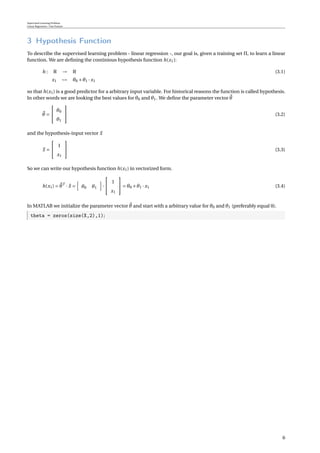
In MATLAB we initialize the descent algorithm with our given input matrix X, given output matrix Y and an arbitrary
parameter vector θ. At the beginning we need to initialize the iteration steps iter and the learning rate alpha. To
check if our learning algorithm is working well we will calculate stepwise the value of our cost function. For this
reason we initialize a cost-converge-test function J_test. After the gradient descent algorithm is done we plot the
cost-converge-test function dependending on the iteration steps iters.
iter = 1000;
alpha = 0.01;
J_test = zeros(iter,1);
iters =[1:1:iter]’;
for k=1:iter
J_test(k) = 1/(2*m) * sum( (X*theta - Y).ˆ2 );
theta_temp1 = theta(1) - alpha*1/m * sum( X*theta - Y );
theta_temp2 = theta(2) - alpha*1/m * sum( (X*theta - Y ).*X(:,2) );
theta(1) = theta_temp1;
theta(2) = theta_temp2;
end
plot(k,J_test)
disp([’theta_0: ’, num2str(theta(1)),’ ; theta_1: ’,num2str(theta(2))])
10

11. Supervised Learning Problem
Linear Regression / One Feature
6 Normal Equation Algorithm (Alternative)
Gradient descent gives one way of minimizing J(θ0,θ1). Let’s discuss a second way of doing so, this time performing
the minimization explicitly and without resorting to an iterative algorithm. In the "Normal Equation" method, we will
minimize J(θ0,θ1) by explicitly taking its derivatives with respect to the θj ’s, and setting them to zero. This allows us
to find the optimum theta without iteration. The normal equation formula is given below:
θ = (X ·X)−1
·X ·Y (6.1)
With the normal equation, computing the inversion has complexity O(n3
). So if we have a very large number of
features, the normal equation will be slow. In practice, when n exceeds 10,000 it might be a good time to go from a
normal solution to an iterative process.
In MATLAB we write
theta = inv(X’*X)*X’*Y;
11

12. Supervised Learning Problem
Linear Regression / One Feature
7 Important Conclusions
• Gradient Descent Algorithm
– Need to choose α
– Needs many iterations O(kn2
)
– Works well when n is large
– if α is too small, gradient descent can be slow
– if α is too large, gradient descent can overshoot the minimum. It may be fail to converge, or even diverge
• Normal Equation Algorithm
– No need to choose α
– No need to iterate
– O(n3
), need to calculate inverse of (X · X)
– Slow if n is very large
– When implementing the normal equation in MATLAB we want to use the pinv function rather than inv.
The pinv function will give you a value of θ even if (X · X) is not invertible.
– If (X · X) is noninvertible, the common causes might be having
* Redundant features, where two features are very closely related (i.e. they are linearly dependent)
* Too many features (e.g. m ≤ n). In this case, delete some features or use regularization (see other
journal).
12

13. Supervised Learning Problem
Linear Regression / One Feature
Glossary
Ω Input set
Υ Output set
x0 Bias element
x1 Feature element
y1 Output element
u Arbitrary element in the input set
v Arbitrary element in the output set
m Number of feature examples
Π Training set
t(x(i)
1 ) Training function (discrete)
T Training matrix
X Input matrix
Y Output matrix
h(x1) Hypothesis function (continuous)
θ0 1-st element of the parameter vector
θ1 2-nd element of the parameter vector
θj j-th element of the parameter vector
θ Parameter vector
x Hypothesis-input vector
13

14. Supervised Learning Problem
Linear Regression / One Feature
J(θ0,θ1) Cost function
x(i)
1 i-th feature value
y(i)
1 i-th output value
α Learning rate
∂
∂θj
J(θ0,θ1) Partial derivative of the cost function
X Transpose of the input matrix
n Number of feature elements
14