SlideShare a Scribd company logo
1 of 13
Download to read offline
Introduction to
functions
mc-TY-introfns-2009-1
A function is a rule which operates on one number to give another number. However, not every
rule describes a valid function. This unit explains how to see whether a given rule describes a
valid function, and introduces some of the mathematical terms associated with functions.
In order to master the techniques explained here it is vital that you undertake plenty of practice
exercises so that they become second nature.
After reading this text, and/or viewing the video tutorial on this topic, you should be able to:
• recognise when a rule describes a valid function,
• be able to plot the graph of a part of a function,
• find a suitable domain for a function, and find the corresponding range.
Contents
1. What is a function? 2
2. Plotting the graph of a function 3
3. When is a function valid? 4
4. Some further examples 6
www.mathcentre.ac.uk 1 c mathcentre 2009
1. What is a function?
Here is a definition of a function.
A function is a rule which maps a number to another unique number.
In other words, if we start off with an input, and we apply the function, we get an output.
For example, we might have a function that added 3 to any number. So if we apply this function
to the number 2, we get the number 5. If we apply this function to the number 8, we get the
number 11. If we apply this function to the number x, we get the number x + 3.
We can show this mathematically by writing
f(x) = x + 3.
The number x that we use for the input of the function is called the argument of the function.
So if we choose an argument of 2, we get
f(2) = 2 + 3 = 5.
If we choose an argument of 8, we get
f(8) = 8 + 3 = 11.
If we choose an argument of −6, we get
f(−6) = −6 + 3 = −3.
If we choose an argument of z, we get
f(z) = z + 3.
If we choose an argument of x2
, we get
f(x2
) = x2
+ 3.
At first sight, it seems that we can pick any number we choose for the argument. However, that
is not the case, as we shall see later. But because we do have some choice in the number we
can pick, we call the argument the independent variable. The output of the function, e.g. f(x),
f(5), etc. depends upon the argument, and so this is called the dependent variable.
Key Point
A function is a rule that maps a number to another unique number.
The input to the function is called the independent variable, and is also called the argument of
the function. The output of the function is called the dependent variable.
www.mathcentre.ac.uk 2 c mathcentre 2009
2. Plotting the graph of a function
If we have a function given by a formula, we can try to plot its graph. Suppose, for example,
that we have a function f defined by
f(x) = 3x2
− 4.
The argument of the function (the independent variable) is x, and the output (the dependent
variable) is 3x2
− 4. So we can calculate the output of the function for different arguments:
f(0) = 3 × 02
− 4 = −4
f(1) = 3 × 12
− 4 = −1
f(2) = 3 × 22
− 4 = 8
f(−1) = 3 × (−1)2
− 4 = −1
f(−2) = 3 × (−2)2
− 4 = 8.
We can put this information into a table to help us plot the graph of the function.
x f(x)
−2 8
−1 −1
0 −4
1 −1
2 8
f(x)
x−2 1 2−1
8
4
−4
We can use the graph of the function to find the output corresponding to a given argument. For
instance, if we have an argument of 2, we start on the horizontal axis at the point where x = 2,
and we follow the line up until we reach the graph. Then we follow the line across so that we
can read off the value of f(x) on the vertical axis. In this case, the value of f(x) is 8. Of course
we already know this, because x = 2 is one of the values in our table.
f(x)
x−2 1 2−1
8
4
−4
www.mathcentre.ac.uk 3 c mathcentre 2009
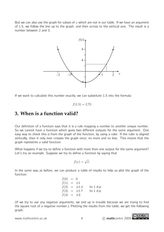
But we can also use the graph for values of x which are not in our table. If we have an argument
of 1.5, we follow the line up to the graph, and then across to the vertical axis. The result is a
number between 2 and 3.
f(x)
x−2 1 2−1
8
4
−4
If we want to calculate this number exactly, we can substitute 1.5 into the formula:
f(1.5) = 2.75
3. When is a function valid?
Our definition of a function says that it is a rule mapping a number to another unique number.
So we cannot have a function which gives two different outputs for the same argument. One
easy way to check this is from the graph of the function, by using a ruler. If the ruler is aligned
vertically, then it only ever crosses the graph once; no more and no less. This means that the
graph represents a valid function.
What happens if we try to define a function with more than one output for the same argument?
Let’s try an example. Suppose we try to define a function by saying that
f(x) =
√
x.
In the same way as before, we can produce a table of results to help us plot the graph of the
function:
f(0) = 0
f(1) = ±1
f(2) = ±1.4 to 1 d.p.
f(3) = ±1.7 to 1 d.p.
f(4) = ±2.
(If we try to use any negative arguments, we end up in trouble because we are trying to find
the square root of a negative number.) Plotting the results from the table, we get the following
graph.
www.mathcentre.ac.uk 4 c mathcentre 2009
f(x)
x2 3 41
2
−1
1
−2
ruler
Using the ruler, it is quite clear that there are two values for all of the positive arguments. So
as it stands, this is not a valid function.
One way around this problem is to define
√
x to take only the positive values, or zero: this is
sometimes called the positive square root of x. However, there is still the issue that we cannot
choose a negative argument. So we should also choose to restrict the choice of argument to
positive values, or zero.
f(x)
x2 3 41
2
1
When considering these kinds of restrictions, it is important to use the right mathematical
language. We say that the set of possible inputs is called the domain of the function, and the set
of corresponding outputs is called the range. In the example above, we have defined the function
as follows:
f(x) =
√
x x ≥ 0, f(x) ≥ 0,
so that the domain of the function is the set of numbers x ≥ 0, and the range is the corresponding
set of numbers f(x) ≥ 0.
Key Point
The domain of a function is the set of possible inputs. The range of a function is the set of
corresponding outputs.
www.mathcentre.ac.uk 5 c mathcentre 2009
4. Some further examples
Example
Consider the function
f(x) = 2x2
− 3x + 5.
To make sure that the function is valid, we need to check whether we get exactly one output
for each input, and whether there needs to be any restriction on the domain. As before, we can
calculate the output of this function at some specific values to help us with plotting our graph:
f(0) = 2 × 02
− 3 × 0 + 5
= 5,
f(1) = 2 × 12
− 3 × 1 + 5
= 2 − 3 + 5
= 4,
f(2) = 2 × 22
− 3 × 2 + 5
= 8 − 6 + 5
= 7,
f(3) = 2 × 32
− 3 × 3 + 5
= 18 − 9 + 5
= 14,
f(−1) = 2 × (−1)2
− 3 × (−1) + 5
= 2 + 3 + 5
= 10.
Now we can put this into a table, and plot the graph.
x f(x)
−1 10
0 5
1 4
2 7
3 14
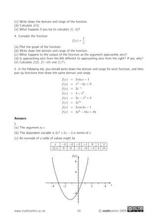
14
10
5
1 2 3-1
f(x)
x
www.mathcentre.ac.uk 6 c mathcentre 2009
A vertical ruler always crosses the graph once, and so the domain needs no restrictions, and
the function is valid. We can also see from the graph that the minimum output occurs when
x = 0.75, and that is when f(x) = 3.875. So the range of the function is f(x) ≥ 3.875.
Example
What about the function
f(x) =
1
x
?
As usual, the first step is to check some values.
f(1) = 1, f(2) = 1
2
, f(3) = 1
3
, f(4) = 1
4
,
f(−1) =
1
(−1)
= −1, f(−2) =
1
(−2)
= −1
2
,
f(−3) =
1
(−3)
= −1
3
, f(−4) =
1
(−4)
= −1
4
.
When we try to calculate f(0) we have a problem, because we cannot divide by zero. So we
have to restrict the domain to exclude x = 0.
f(x)
x−1−2 1 2 3 4−3−4
1
1
2
1
2
−
−1
Because of this problem when x = 0, we have to restrict the domain to make the function valid.
You can also see from the graph that there is no value of x where f(x) = 0, so zero is also
excluded from the range. The function is therefore defined by
f(x) = 1/x x = 0, f(x) = 0.
You might want to know what exactly is going on at this point when x = 0. One way to find
out is to look at what is happening very close to zero. So let’s try some positive values for the
argument getting closer and closer to zero, in order to see what happens:
f(1) = 1, f
1
2
=
1
1/2
= 2, f
1
10
=
1
1/10
= 10,
f
1
1,000
=
1
1/1,000
= 1,000, f
1
1,000,000
=
1
1/1,000,000
= 1,000,000 .
So you can see that as we approach zero from the right, the output approaches infinity.
www.mathcentre.ac.uk 7 c mathcentre 2009
Now let’s try some negative values for the argument, getting closer and closer to zero from the
left-hand side, in order to see what happens:
f(−1) =
1
(−1)
= −1, f −
1
2
=
1
(−1/2)
= −2, f −
1
10
=
1
(−1/10)
= −10,
f −
1
1,000
=
1
(−1/1,000)
= −1,000, f −
1
1,000,000
=
1
(−1/1,000,000)
= −1,000,000 .
You can see that as we approach zero from the left, the output approaches negative infinity. So
in this case, approaching zero from the left is very different from approaching it from the right.
Example
For our final example, take the function
f(x) =
1
(x − 2)2
.
As usual, we must calculate some values:
f(−2) =
1
(−2 − 2)2
= 1
16
f(−1) =
1
(−1 − 2)2
= 1
9
f(0) =
1
(0 − 2)2
= 1
4
f(1) =
1
(1 − 2)2
= 1
f(2) =
1
(2 − 2)2
= dividing by zero
f(3) =
1
(3 − 2)2
= 1
f(4) =
1
(4 − 2)2
= 1
4
f(5) =
1
(5 − 2)2
= 1
9
f(6) =
1
(6 − 2)2
= 1
16
.
Now we can construct a table, and plot the graph of the function.
x f(x)
−2 1
16
−1 1
9
0 1
4
1 1
2 dividing by zero
3 1
4 1
4
5 1
9
6 1
16
www.mathcentre.ac.uk 8 c mathcentre 2009
f(x)
x
1 2 3 4 5 6−1−2
1
1
4
3
4
1
2
The vertical line at x = 2 is called an asymptote; it is a line which is approached by the graph but
never reached. Although it is clear that we will have to omit x = 2 from the domain, this time the
situation is slightly different. You can see that at either side of x = 2, f(x) is approaching infinity.
You should also notice that we cannot have any negative values for f(x), or even f(x) = 0. So
we have to define our function as
f(x) =
1
(x − 2)2
x = 2, f(x) > 0.
Exercises
1. Consider the function
f(x) = 2x2
+ 5x − 3.
(a) Write down the argument of this function.
(b) Write down the dependent variable in terms of the argument.
(c) Use a table of values to help you plot the graph of the function.
(d) From your graph, estimate f(1.5).
(e) Use your function to calculate f(1.5) exactly.
(f) Write down the domain and range of the function.
(g) Re-write the function with argument y.
2. Consider the function
f(x) =
1
(x − 3)2
.
(a) Plot the graph of the function.
(b) Write down the domain and range of the function.
(c) Re-write the function with argument z.
(d) Use your graph to estimate f(1).
(e) Use the function to calculate f(1) exactly.
(f) Write down another function where x = 4 has to be omitted from the domain.
3. Consider the function
f(x) = 3
√
x.
(a) What assumptions must be made about the function to ensure validity?
(b) Plot the graph of the function.
www.mathcentre.ac.uk 9 c mathcentre 2009
(c) Write down the domain and range of the function.
(d) Calculate f(3).
(e) What happens if you try to calculate f(−2)?
4. Consider the function
f(x) =
1
x
.
(a) Plot the graph of the function.
(b) Write down the domain and range of the function.
(c) What happens to the output of the function as the argument approaches zero?
(d) Is approaching zero from the left different to approaching zero from the right? If yes, why?
(e) Calculate f(2), f(−10) and f(z3
).
5. In the following list, you should write down the domain and range for each function, and then
pair up functions that share the same domain and range.
f(x) = 2 sin x − 1
f(x) = x2
− 6x + 9
f(x) = 2e−x
f(x) = 4 − x2
f(x) = 2x − x2
+ 3
f(x) = 3e5x
f(x) = 2 cos 2x − 1
f(x) = 4x2
− 16x + 16
Answers
1.
(a) The argument is x.
(b) The dependent variable is 2x2
+ 5x − 3 in terms of x.
(c) An example of a table of values might be
x −4 −3 −2 −1 0 1 2
f(x) 9 0 −5 −6 −3 4 15
f(x)
x−4 2 4−2
8
4
−4
www.mathcentre.ac.uk 10 c mathcentre 2009
(d) Draw a line up from x = 1.5, and read off the value on the y-axis.
(e) f(1.5) = 9.
(f) Reading off from the graph, f(x) ≥ −6.125, and also −∞ < x < ∞.
(g) The function is f(y) = 2y2
+ 5y − 3 using an argument y.
www.mathcentre.ac.uk 11 c mathcentre 2009
2.
(a)
f(x)
x2 4 6 8−2
6
4
2
(b) The domain is x = 3, the range is f(x) > 0.
(c) The function is f(z) =
1
(z − 3)2
using an argument z.
(d) Draw a line up from x = 1, and read off the value on the y-axis.
(e) f(1) =
1
(1 − 3)2
= 1
4
.
(f) One such function is f(x) =
1
(x − 4)2
, but there are many others.
3.
(a) We must assume that we take the positive square root, and that we take x ≥ 0.
(b)
f(x)
x5 10 15−5
10
5
(c) The domain is x ≥ 0, the range is f(x) ≥ 0.
(d) f(3) = 3
√
3 = 5.2 (to 1 d.p.).
(e) If you try to calculate f(−2), you will be attempting to find the square root of a negative
number. This has no real solutions.
www.mathcentre.ac.uk 12 c mathcentre 2009
4.
(a)
f(x)
x
−2−4
2 4 6 8
4
−2
−4
2
−8 −6
(b) The domain is x = 0, the range is f(x) = 0.
(c) The output approaches ±∞.
(d) Approaching from the left is different to approaching from the right. Approaching from the
left, the output decreases rapidly to negative infinity. Approaching from the right, the output
increases rapidly to positive infinity.
(e) f(2) = 1
2
, f(−10) = − 1
10
, f(z3
) = 1/z3
.
5.
domain range
f(x) = 2 sin x − 1 −∞ < x < ∞ −3 ≤ f(x) ≤ 1
f(x) = x2
− 6x + 9 −∞ < x < ∞ f(x) ≥ 0
f(x) = 2e−x
−∞ < x < ∞ f(x) > 0
f(x) = 4 − x2
−∞ < x < ∞ f(x) ≤ 4
f(x) = 2x − x2
+ 3 −∞ < x < ∞ f(x) ≤ 4
f(x) = 3e5x
−∞ < x < ∞ f(x) > 0
f(x) = 2 cos 2x − 1 −∞ < x < ∞ −3 ≤ f(x) ≤ 1
f(x) = 4x2
− 16x + 16 −∞ < x < ∞ f(x) ≥ 0
So the pairs are
f(x) = 2 sin(x) − 1 and f(x) = 2 cos 2x − 1 ,
f(x) = x2
− 6x + 9 and f(x) = 4x2
− 16x + 16 ,
f(x) = 2e−x
and f(x) = 3e5x
,
f(x) = 4 − x2
and f(x) = 2x − x2
+ 3 .
www.mathcentre.ac.uk 13 c mathcentre 2009

More Related Content

What's hot

Functions and its Applications in Mathematics
Functions and its Applications in MathematicsFunctions and its Applications in Mathematics
Functions and its Applications in MathematicsAmit Amola
 
Maths iii quick review by Dr Asish K Mukhopadhyay
Maths iii quick review by Dr Asish K MukhopadhyayMaths iii quick review by Dr Asish K Mukhopadhyay
Maths iii quick review by Dr Asish K MukhopadhyayDr. Asish K Mukhopadhyay
 
Calculus - Functions Review
Calculus - Functions ReviewCalculus - Functions Review
Calculus - Functions Reviewhassaanciit
 
Algebra 2 Section 4-5
Algebra 2 Section 4-5Algebra 2 Section 4-5
Algebra 2 Section 4-5Jimbo Lamb
 
L2 graphs piecewise, absolute,and greatest integer
L2 graphs  piecewise, absolute,and greatest integerL2 graphs  piecewise, absolute,and greatest integer
L2 graphs piecewise, absolute,and greatest integerJames Tagara
 
Math 4 lecture on Graphing Rational Functions
Math 4 lecture on Graphing Rational FunctionsMath 4 lecture on Graphing Rational Functions
Math 4 lecture on Graphing Rational FunctionsLeo Crisologo
 
The Exponential and natural log functions
The Exponential and natural log functionsThe Exponential and natural log functions
The Exponential and natural log functionsJJkedst
 
Notes - Graphs of Polynomials
Notes - Graphs of PolynomialsNotes - Graphs of Polynomials
Notes - Graphs of PolynomialsLori Rapp
 
Functions and graphs
Functions and graphsFunctions and graphs
Functions and graphsSujata Tapare
 
2.2 Polynomial Function Notes
2.2 Polynomial Function Notes2.2 Polynomial Function Notes
2.2 Polynomial Function Noteslgemgnani
 
Module 2 lesson 4 notes
Module 2 lesson 4 notesModule 2 lesson 4 notes
Module 2 lesson 4 notestoni dimella
 
Polynomial functionsandgraphs
Polynomial functionsandgraphsPolynomial functionsandgraphs
Polynomial functionsandgraphsJerlyn Fernandez
 
Piecewise Functions
Piecewise FunctionsPiecewise Functions
Piecewise Functionsswartzje
 

What's hot (20)

Functions and its Applications in Mathematics
Functions and its Applications in MathematicsFunctions and its Applications in Mathematics
Functions and its Applications in Mathematics
 
Maths iii quick review by Dr Asish K Mukhopadhyay
Maths iii quick review by Dr Asish K MukhopadhyayMaths iii quick review by Dr Asish K Mukhopadhyay
Maths iii quick review by Dr Asish K Mukhopadhyay
 
Calculus - Functions Review
Calculus - Functions ReviewCalculus - Functions Review
Calculus - Functions Review
 
Algebra 2 Section 4-5
Algebra 2 Section 4-5Algebra 2 Section 4-5
Algebra 2 Section 4-5
 
L2 graphs piecewise, absolute,and greatest integer
L2 graphs  piecewise, absolute,and greatest integerL2 graphs  piecewise, absolute,and greatest integer
L2 graphs piecewise, absolute,and greatest integer
 
Numerical method (curve fitting)
Numerical method (curve fitting)Numerical method (curve fitting)
Numerical method (curve fitting)
 
Functions
FunctionsFunctions
Functions
 
Math 4 lecture on Graphing Rational Functions
Math 4 lecture on Graphing Rational FunctionsMath 4 lecture on Graphing Rational Functions
Math 4 lecture on Graphing Rational Functions
 
The Exponential and natural log functions
The Exponential and natural log functionsThe Exponential and natural log functions
The Exponential and natural log functions
 
Notes - Graphs of Polynomials
Notes - Graphs of PolynomialsNotes - Graphs of Polynomials
Notes - Graphs of Polynomials
 
Functions and graphs
Functions and graphsFunctions and graphs
Functions and graphs
 
2.2 Polynomial Function Notes
2.2 Polynomial Function Notes2.2 Polynomial Function Notes
2.2 Polynomial Function Notes
 
Es272 ch5b
Es272 ch5bEs272 ch5b
Es272 ch5b
 
FUNCTION AND RELATION
FUNCTION AND RELATIONFUNCTION AND RELATION
FUNCTION AND RELATION
 
Polynomial functions
Polynomial functionsPolynomial functions
Polynomial functions
 
Module 2 lesson 4 notes
Module 2 lesson 4 notesModule 2 lesson 4 notes
Module 2 lesson 4 notes
 
Polynomial functionsandgraphs
Polynomial functionsandgraphsPolynomial functionsandgraphs
Polynomial functionsandgraphs
 
Matlab lecture 5 bisection method@taj
Matlab lecture 5  bisection method@tajMatlab lecture 5  bisection method@taj
Matlab lecture 5 bisection method@taj
 
Lagrange’s interpolation formula
Lagrange’s interpolation formulaLagrange’s interpolation formula
Lagrange’s interpolation formula
 
Piecewise Functions
Piecewise FunctionsPiecewise Functions
Piecewise Functions
 

Viewers also liked (7)

Chap 4 complex numbers focus exam ace
Chap 4 complex numbers focus exam aceChap 4 complex numbers focus exam ace
Chap 4 complex numbers focus exam ace
 
Compacting form2baru
Compacting form2baruCompacting form2baru
Compacting form2baru
 
Pencapaian2011
Pencapaian2011Pencapaian2011
Pencapaian2011
 
Chapter 2 sequencess and series
Chapter 2 sequencess and seriesChapter 2 sequencess and series
Chapter 2 sequencess and series
 
Kertas model pep sebenar (pmr)
Kertas model pep sebenar (pmr)Kertas model pep sebenar (pmr)
Kertas model pep sebenar (pmr)
 
Ayat ayat al quran tentang akhlak
Ayat  ayat al quran tentang akhlakAyat  ayat al quran tentang akhlak
Ayat ayat al quran tentang akhlak
 
Panduan penulisan kajian tingkatan 6 (1)
Panduan  penulisan kajian tingkatan 6 (1)Panduan  penulisan kajian tingkatan 6 (1)
Panduan penulisan kajian tingkatan 6 (1)
 

Similar to Note introductions of functions

Introduction to Functions
Introduction to FunctionsIntroduction to Functions
Introduction to FunctionsMelanie Loslo
 
Relations and functions
Relations and functions Relations and functions
Relations and functions Nabeel Simair
 
Chapter on Functions and Graphs.ppt
Chapter on Functions and Graphs.pptChapter on Functions and Graphs.ppt
Chapter on Functions and Graphs.pptPhongLan30
 
237654933 mathematics-t-form-6
237654933 mathematics-t-form-6237654933 mathematics-t-form-6
237654933 mathematics-t-form-6homeworkping3
 
Calculus 1 Lecture Notes (Functions and Their Graphs)
Calculus 1 Lecture Notes (Functions and Their Graphs)Calculus 1 Lecture Notes (Functions and Their Graphs)
Calculus 1 Lecture Notes (Functions and Their Graphs)Mohammed Matar
 
3 2 Polynomial Functions And Their Graphs
3 2 Polynomial Functions And Their Graphs3 2 Polynomial Functions And Their Graphs
3 2 Polynomial Functions And Their Graphssilvia
 
Functions and Relations
Functions and RelationsFunctions and Relations
Functions and RelationsJailah13
 
Lesson 2 - Functions and their Graphs - NOTES.ppt
Lesson 2 - Functions and their Graphs - NOTES.pptLesson 2 - Functions and their Graphs - NOTES.ppt
Lesson 2 - Functions and their Graphs - NOTES.pptJaysonMagalong
 
Module 1 quadratic functions
Module 1   quadratic functionsModule 1   quadratic functions
Module 1 quadratic functionsdionesioable
 
Edsc 304 lesson 1
Edsc 304 lesson 1Edsc 304 lesson 1
Edsc 304 lesson 1urenaa
 
Generating functions (albert r. meyer)
Generating functions (albert r. meyer)Generating functions (albert r. meyer)
Generating functions (albert r. meyer)Ilir Destani
 
Mathematics 9 Quadratic Functions (Module 1)
Mathematics 9 Quadratic Functions (Module 1)Mathematics 9 Quadratic Functions (Module 1)
Mathematics 9 Quadratic Functions (Module 1)Juan Miguel Palero
 
Storyboard math
Storyboard mathStoryboard math
Storyboard mathshandex
 

Similar to Note introductions of functions (20)

Introduction to Functions
Introduction to FunctionsIntroduction to Functions
Introduction to Functions
 
mc-ty-polynomial-2009-1.pdf
mc-ty-polynomial-2009-1.pdfmc-ty-polynomial-2009-1.pdf
mc-ty-polynomial-2009-1.pdf
 
.
..
.
 
Functions
FunctionsFunctions
Functions
 
Relations and functions
Relations and functions Relations and functions
Relations and functions
 
Chapter on Functions and Graphs.ppt
Chapter on Functions and Graphs.pptChapter on Functions and Graphs.ppt
Chapter on Functions and Graphs.ppt
 
237654933 mathematics-t-form-6
237654933 mathematics-t-form-6237654933 mathematics-t-form-6
237654933 mathematics-t-form-6
 
function
functionfunction
function
 
Calculus 1 Lecture Notes (Functions and Their Graphs)
Calculus 1 Lecture Notes (Functions and Their Graphs)Calculus 1 Lecture Notes (Functions and Their Graphs)
Calculus 1 Lecture Notes (Functions and Their Graphs)
 
3 2 Polynomial Functions And Their Graphs
3 2 Polynomial Functions And Their Graphs3 2 Polynomial Functions And Their Graphs
3 2 Polynomial Functions And Their Graphs
 
Functions and Relations
Functions and RelationsFunctions and Relations
Functions and Relations
 
Lesson 2 - Functions and their Graphs - NOTES.ppt
Lesson 2 - Functions and their Graphs - NOTES.pptLesson 2 - Functions and their Graphs - NOTES.ppt
Lesson 2 - Functions and their Graphs - NOTES.ppt
 
Fst ch3 notes
Fst ch3 notesFst ch3 notes
Fst ch3 notes
 
Module 1 quadratic functions
Module 1   quadratic functionsModule 1   quadratic functions
Module 1 quadratic functions
 
7 functions
7   functions7   functions
7 functions
 
Edsc 304 lesson 1
Edsc 304 lesson 1Edsc 304 lesson 1
Edsc 304 lesson 1
 
Generating functions (albert r. meyer)
Generating functions (albert r. meyer)Generating functions (albert r. meyer)
Generating functions (albert r. meyer)
 
Goldie chapter 4 function
Goldie chapter 4 functionGoldie chapter 4 function
Goldie chapter 4 function
 
Mathematics 9 Quadratic Functions (Module 1)
Mathematics 9 Quadratic Functions (Module 1)Mathematics 9 Quadratic Functions (Module 1)
Mathematics 9 Quadratic Functions (Module 1)
 
Storyboard math
Storyboard mathStoryboard math
Storyboard math
 

Recently uploaded

How to Manage Global Discount in Odoo 17 POS
How to Manage Global Discount in Odoo 17 POSHow to Manage Global Discount in Odoo 17 POS
How to Manage Global Discount in Odoo 17 POSCeline George
 
Google Gemini An AI Revolution in Education.pptx
Google Gemini An AI Revolution in Education.pptxGoogle Gemini An AI Revolution in Education.pptx
Google Gemini An AI Revolution in Education.pptxDr. Sarita Anand
 
Accessible Digital Futures project (20/03/2024)
Accessible Digital Futures project (20/03/2024)Accessible Digital Futures project (20/03/2024)
Accessible Digital Futures project (20/03/2024)Jisc
 
Python Notes for mca i year students osmania university.docx
Python Notes for mca i year students osmania university.docxPython Notes for mca i year students osmania university.docx
Python Notes for mca i year students osmania university.docxRamakrishna Reddy Bijjam
 
Unit 3 Emotional Intelligence and Spiritual Intelligence.pdf
Unit 3 Emotional Intelligence and Spiritual Intelligence.pdfUnit 3 Emotional Intelligence and Spiritual Intelligence.pdf
Unit 3 Emotional Intelligence and Spiritual Intelligence.pdfDr Vijay Vishwakarma
 
21st_Century_Skills_Framework_Final_Presentation_2.pptx
21st_Century_Skills_Framework_Final_Presentation_2.pptx21st_Century_Skills_Framework_Final_Presentation_2.pptx
21st_Century_Skills_Framework_Final_Presentation_2.pptxJoelynRubio1
 
FSB Advising Checklist - Orientation 2024
FSB Advising Checklist - Orientation 2024FSB Advising Checklist - Orientation 2024
FSB Advising Checklist - Orientation 2024Elizabeth Walsh
 
REMIFENTANIL: An Ultra short acting opioid.pptx
REMIFENTANIL: An Ultra short acting opioid.pptxREMIFENTANIL: An Ultra short acting opioid.pptx
REMIFENTANIL: An Ultra short acting opioid.pptxDr. Ravikiran H M Gowda
 
How to Add a Tool Tip to a Field in Odoo 17
How to Add a Tool Tip to a Field in Odoo 17How to Add a Tool Tip to a Field in Odoo 17
How to Add a Tool Tip to a Field in Odoo 17Celine George
 
COMMUNICATING NEGATIVE NEWS - APPROACHES .pptx
COMMUNICATING NEGATIVE NEWS - APPROACHES .pptxCOMMUNICATING NEGATIVE NEWS - APPROACHES .pptx
COMMUNICATING NEGATIVE NEWS - APPROACHES .pptxannathomasp01
 
Basic Intentional Injuries Health Education
Basic Intentional Injuries Health EducationBasic Intentional Injuries Health Education
Basic Intentional Injuries Health EducationNeilDeclaro1
 
latest AZ-104 Exam Questions and Answers
latest AZ-104 Exam Questions and Answerslatest AZ-104 Exam Questions and Answers
latest AZ-104 Exam Questions and Answersdalebeck957
 
HMCS Vancouver Pre-Deployment Brief - May 2024 (Web Version).pptx
HMCS Vancouver Pre-Deployment Brief - May 2024 (Web Version).pptxHMCS Vancouver Pre-Deployment Brief - May 2024 (Web Version).pptx
HMCS Vancouver Pre-Deployment Brief - May 2024 (Web Version).pptxmarlenawright1
 
HMCS Max Bernays Pre-Deployment Brief (May 2024).pptx
HMCS Max Bernays Pre-Deployment Brief (May 2024).pptxHMCS Max Bernays Pre-Deployment Brief (May 2024).pptx
HMCS Max Bernays Pre-Deployment Brief (May 2024).pptxEsquimalt MFRC
 
Food safety_Challenges food safety laboratories_.pdf
Food safety_Challenges food safety laboratories_.pdfFood safety_Challenges food safety laboratories_.pdf
Food safety_Challenges food safety laboratories_.pdfSherif Taha
 
Single or Multiple melodic lines structure
Single or Multiple melodic lines structureSingle or Multiple melodic lines structure
Single or Multiple melodic lines structuredhanjurrannsibayan2
 
SOC 101 Demonstration of Learning Presentation
SOC 101 Demonstration of Learning PresentationSOC 101 Demonstration of Learning Presentation
SOC 101 Demonstration of Learning Presentationcamerronhm
 
How to setup Pycharm environment for Odoo 17.pptx
How to setup Pycharm environment for Odoo 17.pptxHow to setup Pycharm environment for Odoo 17.pptx
How to setup Pycharm environment for Odoo 17.pptxCeline George
 
How to Create and Manage Wizard in Odoo 17
How to Create and Manage Wizard in Odoo 17How to Create and Manage Wizard in Odoo 17
How to Create and Manage Wizard in Odoo 17Celine George
 
Understanding Accommodations and Modifications
Understanding  Accommodations and ModificationsUnderstanding  Accommodations and Modifications
Understanding Accommodations and ModificationsMJDuyan
 

Recently uploaded (20)

How to Manage Global Discount in Odoo 17 POS
How to Manage Global Discount in Odoo 17 POSHow to Manage Global Discount in Odoo 17 POS
How to Manage Global Discount in Odoo 17 POS
 
Google Gemini An AI Revolution in Education.pptx
Google Gemini An AI Revolution in Education.pptxGoogle Gemini An AI Revolution in Education.pptx
Google Gemini An AI Revolution in Education.pptx
 
Accessible Digital Futures project (20/03/2024)
Accessible Digital Futures project (20/03/2024)Accessible Digital Futures project (20/03/2024)
Accessible Digital Futures project (20/03/2024)
 
Python Notes for mca i year students osmania university.docx
Python Notes for mca i year students osmania university.docxPython Notes for mca i year students osmania university.docx
Python Notes for mca i year students osmania university.docx
 
Unit 3 Emotional Intelligence and Spiritual Intelligence.pdf
Unit 3 Emotional Intelligence and Spiritual Intelligence.pdfUnit 3 Emotional Intelligence and Spiritual Intelligence.pdf
Unit 3 Emotional Intelligence and Spiritual Intelligence.pdf
 
21st_Century_Skills_Framework_Final_Presentation_2.pptx
21st_Century_Skills_Framework_Final_Presentation_2.pptx21st_Century_Skills_Framework_Final_Presentation_2.pptx
21st_Century_Skills_Framework_Final_Presentation_2.pptx
 
FSB Advising Checklist - Orientation 2024
FSB Advising Checklist - Orientation 2024FSB Advising Checklist - Orientation 2024
FSB Advising Checklist - Orientation 2024
 
REMIFENTANIL: An Ultra short acting opioid.pptx
REMIFENTANIL: An Ultra short acting opioid.pptxREMIFENTANIL: An Ultra short acting opioid.pptx
REMIFENTANIL: An Ultra short acting opioid.pptx
 
How to Add a Tool Tip to a Field in Odoo 17
How to Add a Tool Tip to a Field in Odoo 17How to Add a Tool Tip to a Field in Odoo 17
How to Add a Tool Tip to a Field in Odoo 17
 
COMMUNICATING NEGATIVE NEWS - APPROACHES .pptx
COMMUNICATING NEGATIVE NEWS - APPROACHES .pptxCOMMUNICATING NEGATIVE NEWS - APPROACHES .pptx
COMMUNICATING NEGATIVE NEWS - APPROACHES .pptx
 
Basic Intentional Injuries Health Education
Basic Intentional Injuries Health EducationBasic Intentional Injuries Health Education
Basic Intentional Injuries Health Education
 
latest AZ-104 Exam Questions and Answers
latest AZ-104 Exam Questions and Answerslatest AZ-104 Exam Questions and Answers
latest AZ-104 Exam Questions and Answers
 
HMCS Vancouver Pre-Deployment Brief - May 2024 (Web Version).pptx
HMCS Vancouver Pre-Deployment Brief - May 2024 (Web Version).pptxHMCS Vancouver Pre-Deployment Brief - May 2024 (Web Version).pptx
HMCS Vancouver Pre-Deployment Brief - May 2024 (Web Version).pptx
 
HMCS Max Bernays Pre-Deployment Brief (May 2024).pptx
HMCS Max Bernays Pre-Deployment Brief (May 2024).pptxHMCS Max Bernays Pre-Deployment Brief (May 2024).pptx
HMCS Max Bernays Pre-Deployment Brief (May 2024).pptx
 
Food safety_Challenges food safety laboratories_.pdf
Food safety_Challenges food safety laboratories_.pdfFood safety_Challenges food safety laboratories_.pdf
Food safety_Challenges food safety laboratories_.pdf
 
Single or Multiple melodic lines structure
Single or Multiple melodic lines structureSingle or Multiple melodic lines structure
Single or Multiple melodic lines structure
 
SOC 101 Demonstration of Learning Presentation
SOC 101 Demonstration of Learning PresentationSOC 101 Demonstration of Learning Presentation
SOC 101 Demonstration of Learning Presentation
 
How to setup Pycharm environment for Odoo 17.pptx
How to setup Pycharm environment for Odoo 17.pptxHow to setup Pycharm environment for Odoo 17.pptx
How to setup Pycharm environment for Odoo 17.pptx
 
How to Create and Manage Wizard in Odoo 17
How to Create and Manage Wizard in Odoo 17How to Create and Manage Wizard in Odoo 17
How to Create and Manage Wizard in Odoo 17
 
Understanding Accommodations and Modifications
Understanding  Accommodations and ModificationsUnderstanding  Accommodations and Modifications
Understanding Accommodations and Modifications
 

Note introductions of functions

  • 1. Introduction to functions mc-TY-introfns-2009-1 A function is a rule which operates on one number to give another number. However, not every rule describes a valid function. This unit explains how to see whether a given rule describes a valid function, and introduces some of the mathematical terms associated with functions. In order to master the techniques explained here it is vital that you undertake plenty of practice exercises so that they become second nature. After reading this text, and/or viewing the video tutorial on this topic, you should be able to: • recognise when a rule describes a valid function, • be able to plot the graph of a part of a function, • find a suitable domain for a function, and find the corresponding range. Contents 1. What is a function? 2 2. Plotting the graph of a function 3 3. When is a function valid? 4 4. Some further examples 6 www.mathcentre.ac.uk 1 c mathcentre 2009
  • 2. 1. What is a function? Here is a definition of a function. A function is a rule which maps a number to another unique number. In other words, if we start off with an input, and we apply the function, we get an output. For example, we might have a function that added 3 to any number. So if we apply this function to the number 2, we get the number 5. If we apply this function to the number 8, we get the number 11. If we apply this function to the number x, we get the number x + 3. We can show this mathematically by writing f(x) = x + 3. The number x that we use for the input of the function is called the argument of the function. So if we choose an argument of 2, we get f(2) = 2 + 3 = 5. If we choose an argument of 8, we get f(8) = 8 + 3 = 11. If we choose an argument of −6, we get f(−6) = −6 + 3 = −3. If we choose an argument of z, we get f(z) = z + 3. If we choose an argument of x2 , we get f(x2 ) = x2 + 3. At first sight, it seems that we can pick any number we choose for the argument. However, that is not the case, as we shall see later. But because we do have some choice in the number we can pick, we call the argument the independent variable. The output of the function, e.g. f(x), f(5), etc. depends upon the argument, and so this is called the dependent variable. Key Point A function is a rule that maps a number to another unique number. The input to the function is called the independent variable, and is also called the argument of the function. The output of the function is called the dependent variable. www.mathcentre.ac.uk 2 c mathcentre 2009
  • 3. 2. Plotting the graph of a function If we have a function given by a formula, we can try to plot its graph. Suppose, for example, that we have a function f defined by f(x) = 3x2 − 4. The argument of the function (the independent variable) is x, and the output (the dependent variable) is 3x2 − 4. So we can calculate the output of the function for different arguments: f(0) = 3 × 02 − 4 = −4 f(1) = 3 × 12 − 4 = −1 f(2) = 3 × 22 − 4 = 8 f(−1) = 3 × (−1)2 − 4 = −1 f(−2) = 3 × (−2)2 − 4 = 8. We can put this information into a table to help us plot the graph of the function. x f(x) −2 8 −1 −1 0 −4 1 −1 2 8 f(x) x−2 1 2−1 8 4 −4 We can use the graph of the function to find the output corresponding to a given argument. For instance, if we have an argument of 2, we start on the horizontal axis at the point where x = 2, and we follow the line up until we reach the graph. Then we follow the line across so that we can read off the value of f(x) on the vertical axis. In this case, the value of f(x) is 8. Of course we already know this, because x = 2 is one of the values in our table. f(x) x−2 1 2−1 8 4 −4 www.mathcentre.ac.uk 3 c mathcentre 2009
  • 4. But we can also use the graph for values of x which are not in our table. If we have an argument of 1.5, we follow the line up to the graph, and then across to the vertical axis. The result is a number between 2 and 3. f(x) x−2 1 2−1 8 4 −4 If we want to calculate this number exactly, we can substitute 1.5 into the formula: f(1.5) = 2.75 3. When is a function valid? Our definition of a function says that it is a rule mapping a number to another unique number. So we cannot have a function which gives two different outputs for the same argument. One easy way to check this is from the graph of the function, by using a ruler. If the ruler is aligned vertically, then it only ever crosses the graph once; no more and no less. This means that the graph represents a valid function. What happens if we try to define a function with more than one output for the same argument? Let’s try an example. Suppose we try to define a function by saying that f(x) = √ x. In the same way as before, we can produce a table of results to help us plot the graph of the function: f(0) = 0 f(1) = ±1 f(2) = ±1.4 to 1 d.p. f(3) = ±1.7 to 1 d.p. f(4) = ±2. (If we try to use any negative arguments, we end up in trouble because we are trying to find the square root of a negative number.) Plotting the results from the table, we get the following graph. www.mathcentre.ac.uk 4 c mathcentre 2009
  • 5. f(x) x2 3 41 2 −1 1 −2 ruler Using the ruler, it is quite clear that there are two values for all of the positive arguments. So as it stands, this is not a valid function. One way around this problem is to define √ x to take only the positive values, or zero: this is sometimes called the positive square root of x. However, there is still the issue that we cannot choose a negative argument. So we should also choose to restrict the choice of argument to positive values, or zero. f(x) x2 3 41 2 1 When considering these kinds of restrictions, it is important to use the right mathematical language. We say that the set of possible inputs is called the domain of the function, and the set of corresponding outputs is called the range. In the example above, we have defined the function as follows: f(x) = √ x x ≥ 0, f(x) ≥ 0, so that the domain of the function is the set of numbers x ≥ 0, and the range is the corresponding set of numbers f(x) ≥ 0. Key Point The domain of a function is the set of possible inputs. The range of a function is the set of corresponding outputs. www.mathcentre.ac.uk 5 c mathcentre 2009
  • 6. 4. Some further examples Example Consider the function f(x) = 2x2 − 3x + 5. To make sure that the function is valid, we need to check whether we get exactly one output for each input, and whether there needs to be any restriction on the domain. As before, we can calculate the output of this function at some specific values to help us with plotting our graph: f(0) = 2 × 02 − 3 × 0 + 5 = 5, f(1) = 2 × 12 − 3 × 1 + 5 = 2 − 3 + 5 = 4, f(2) = 2 × 22 − 3 × 2 + 5 = 8 − 6 + 5 = 7, f(3) = 2 × 32 − 3 × 3 + 5 = 18 − 9 + 5 = 14, f(−1) = 2 × (−1)2 − 3 × (−1) + 5 = 2 + 3 + 5 = 10. Now we can put this into a table, and plot the graph. x f(x) −1 10 0 5 1 4 2 7 3 14 14 10 5 1 2 3-1 f(x) x www.mathcentre.ac.uk 6 c mathcentre 2009
  • 7. A vertical ruler always crosses the graph once, and so the domain needs no restrictions, and the function is valid. We can also see from the graph that the minimum output occurs when x = 0.75, and that is when f(x) = 3.875. So the range of the function is f(x) ≥ 3.875. Example What about the function f(x) = 1 x ? As usual, the first step is to check some values. f(1) = 1, f(2) = 1 2 , f(3) = 1 3 , f(4) = 1 4 , f(−1) = 1 (−1) = −1, f(−2) = 1 (−2) = −1 2 , f(−3) = 1 (−3) = −1 3 , f(−4) = 1 (−4) = −1 4 . When we try to calculate f(0) we have a problem, because we cannot divide by zero. So we have to restrict the domain to exclude x = 0. f(x) x−1−2 1 2 3 4−3−4 1 1 2 1 2 − −1 Because of this problem when x = 0, we have to restrict the domain to make the function valid. You can also see from the graph that there is no value of x where f(x) = 0, so zero is also excluded from the range. The function is therefore defined by f(x) = 1/x x = 0, f(x) = 0. You might want to know what exactly is going on at this point when x = 0. One way to find out is to look at what is happening very close to zero. So let’s try some positive values for the argument getting closer and closer to zero, in order to see what happens: f(1) = 1, f 1 2 = 1 1/2 = 2, f 1 10 = 1 1/10 = 10, f 1 1,000 = 1 1/1,000 = 1,000, f 1 1,000,000 = 1 1/1,000,000 = 1,000,000 . So you can see that as we approach zero from the right, the output approaches infinity. www.mathcentre.ac.uk 7 c mathcentre 2009
  • 8. Now let’s try some negative values for the argument, getting closer and closer to zero from the left-hand side, in order to see what happens: f(−1) = 1 (−1) = −1, f − 1 2 = 1 (−1/2) = −2, f − 1 10 = 1 (−1/10) = −10, f − 1 1,000 = 1 (−1/1,000) = −1,000, f − 1 1,000,000 = 1 (−1/1,000,000) = −1,000,000 . You can see that as we approach zero from the left, the output approaches negative infinity. So in this case, approaching zero from the left is very different from approaching it from the right. Example For our final example, take the function f(x) = 1 (x − 2)2 . As usual, we must calculate some values: f(−2) = 1 (−2 − 2)2 = 1 16 f(−1) = 1 (−1 − 2)2 = 1 9 f(0) = 1 (0 − 2)2 = 1 4 f(1) = 1 (1 − 2)2 = 1 f(2) = 1 (2 − 2)2 = dividing by zero f(3) = 1 (3 − 2)2 = 1 f(4) = 1 (4 − 2)2 = 1 4 f(5) = 1 (5 − 2)2 = 1 9 f(6) = 1 (6 − 2)2 = 1 16 . Now we can construct a table, and plot the graph of the function. x f(x) −2 1 16 −1 1 9 0 1 4 1 1 2 dividing by zero 3 1 4 1 4 5 1 9 6 1 16 www.mathcentre.ac.uk 8 c mathcentre 2009
  • 9. f(x) x 1 2 3 4 5 6−1−2 1 1 4 3 4 1 2 The vertical line at x = 2 is called an asymptote; it is a line which is approached by the graph but never reached. Although it is clear that we will have to omit x = 2 from the domain, this time the situation is slightly different. You can see that at either side of x = 2, f(x) is approaching infinity. You should also notice that we cannot have any negative values for f(x), or even f(x) = 0. So we have to define our function as f(x) = 1 (x − 2)2 x = 2, f(x) > 0. Exercises 1. Consider the function f(x) = 2x2 + 5x − 3. (a) Write down the argument of this function. (b) Write down the dependent variable in terms of the argument. (c) Use a table of values to help you plot the graph of the function. (d) From your graph, estimate f(1.5). (e) Use your function to calculate f(1.5) exactly. (f) Write down the domain and range of the function. (g) Re-write the function with argument y. 2. Consider the function f(x) = 1 (x − 3)2 . (a) Plot the graph of the function. (b) Write down the domain and range of the function. (c) Re-write the function with argument z. (d) Use your graph to estimate f(1). (e) Use the function to calculate f(1) exactly. (f) Write down another function where x = 4 has to be omitted from the domain. 3. Consider the function f(x) = 3 √ x. (a) What assumptions must be made about the function to ensure validity? (b) Plot the graph of the function. www.mathcentre.ac.uk 9 c mathcentre 2009
  • 10. (c) Write down the domain and range of the function. (d) Calculate f(3). (e) What happens if you try to calculate f(−2)? 4. Consider the function f(x) = 1 x . (a) Plot the graph of the function. (b) Write down the domain and range of the function. (c) What happens to the output of the function as the argument approaches zero? (d) Is approaching zero from the left different to approaching zero from the right? If yes, why? (e) Calculate f(2), f(−10) and f(z3 ). 5. In the following list, you should write down the domain and range for each function, and then pair up functions that share the same domain and range. f(x) = 2 sin x − 1 f(x) = x2 − 6x + 9 f(x) = 2e−x f(x) = 4 − x2 f(x) = 2x − x2 + 3 f(x) = 3e5x f(x) = 2 cos 2x − 1 f(x) = 4x2 − 16x + 16 Answers 1. (a) The argument is x. (b) The dependent variable is 2x2 + 5x − 3 in terms of x. (c) An example of a table of values might be x −4 −3 −2 −1 0 1 2 f(x) 9 0 −5 −6 −3 4 15 f(x) x−4 2 4−2 8 4 −4 www.mathcentre.ac.uk 10 c mathcentre 2009
  • 11. (d) Draw a line up from x = 1.5, and read off the value on the y-axis. (e) f(1.5) = 9. (f) Reading off from the graph, f(x) ≥ −6.125, and also −∞ < x < ∞. (g) The function is f(y) = 2y2 + 5y − 3 using an argument y. www.mathcentre.ac.uk 11 c mathcentre 2009
  • 12. 2. (a) f(x) x2 4 6 8−2 6 4 2 (b) The domain is x = 3, the range is f(x) > 0. (c) The function is f(z) = 1 (z − 3)2 using an argument z. (d) Draw a line up from x = 1, and read off the value on the y-axis. (e) f(1) = 1 (1 − 3)2 = 1 4 . (f) One such function is f(x) = 1 (x − 4)2 , but there are many others. 3. (a) We must assume that we take the positive square root, and that we take x ≥ 0. (b) f(x) x5 10 15−5 10 5 (c) The domain is x ≥ 0, the range is f(x) ≥ 0. (d) f(3) = 3 √ 3 = 5.2 (to 1 d.p.). (e) If you try to calculate f(−2), you will be attempting to find the square root of a negative number. This has no real solutions. www.mathcentre.ac.uk 12 c mathcentre 2009
  • 13. 4. (a) f(x) x −2−4 2 4 6 8 4 −2 −4 2 −8 −6 (b) The domain is x = 0, the range is f(x) = 0. (c) The output approaches ±∞. (d) Approaching from the left is different to approaching from the right. Approaching from the left, the output decreases rapidly to negative infinity. Approaching from the right, the output increases rapidly to positive infinity. (e) f(2) = 1 2 , f(−10) = − 1 10 , f(z3 ) = 1/z3 . 5. domain range f(x) = 2 sin x − 1 −∞ < x < ∞ −3 ≤ f(x) ≤ 1 f(x) = x2 − 6x + 9 −∞ < x < ∞ f(x) ≥ 0 f(x) = 2e−x −∞ < x < ∞ f(x) > 0 f(x) = 4 − x2 −∞ < x < ∞ f(x) ≤ 4 f(x) = 2x − x2 + 3 −∞ < x < ∞ f(x) ≤ 4 f(x) = 3e5x −∞ < x < ∞ f(x) > 0 f(x) = 2 cos 2x − 1 −∞ < x < ∞ −3 ≤ f(x) ≤ 1 f(x) = 4x2 − 16x + 16 −∞ < x < ∞ f(x) ≥ 0 So the pairs are f(x) = 2 sin(x) − 1 and f(x) = 2 cos 2x − 1 , f(x) = x2 − 6x + 9 and f(x) = 4x2 − 16x + 16 , f(x) = 2e−x and f(x) = 3e5x , f(x) = 4 − x2 and f(x) = 2x − x2 + 3 . www.mathcentre.ac.uk 13 c mathcentre 2009