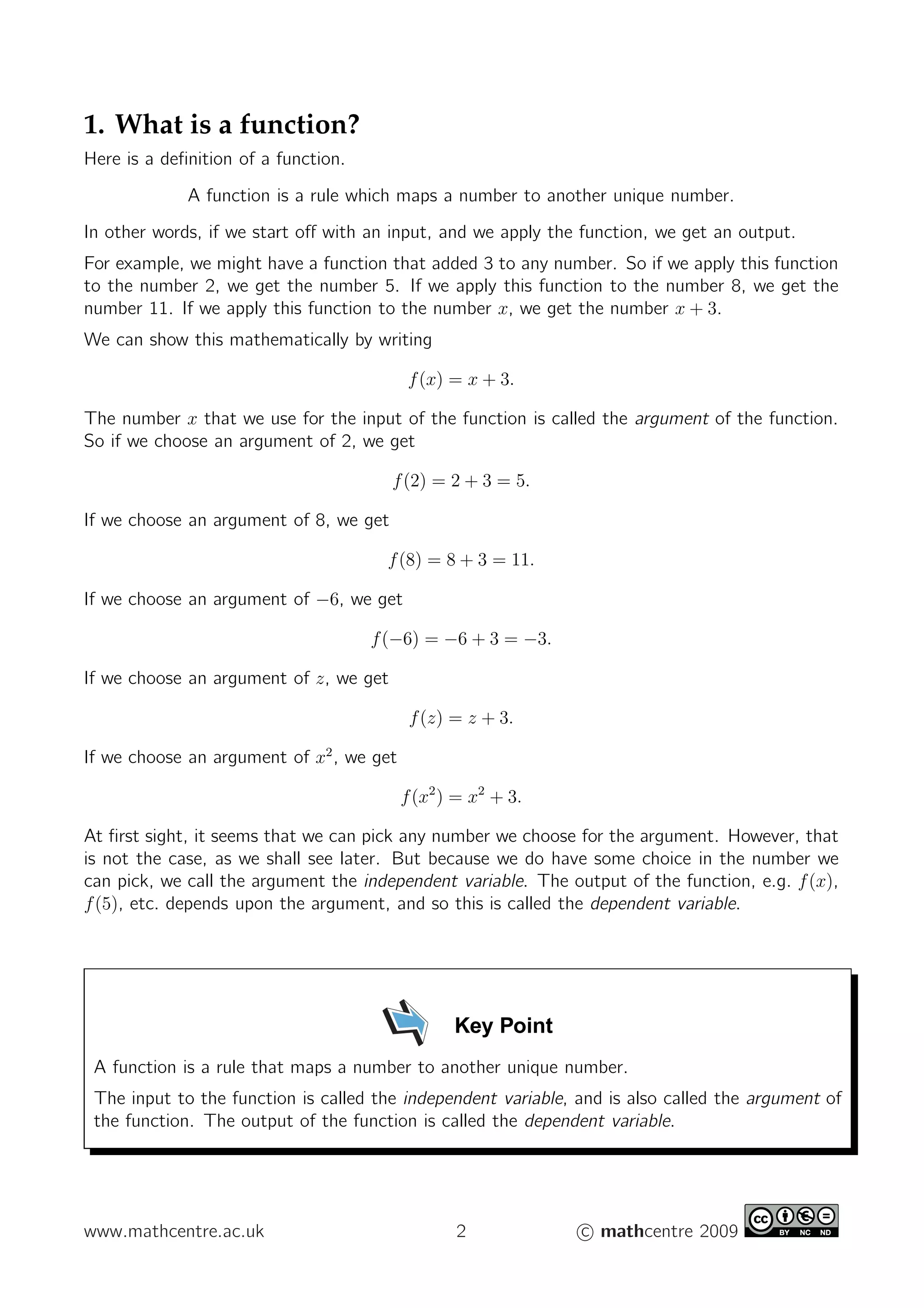
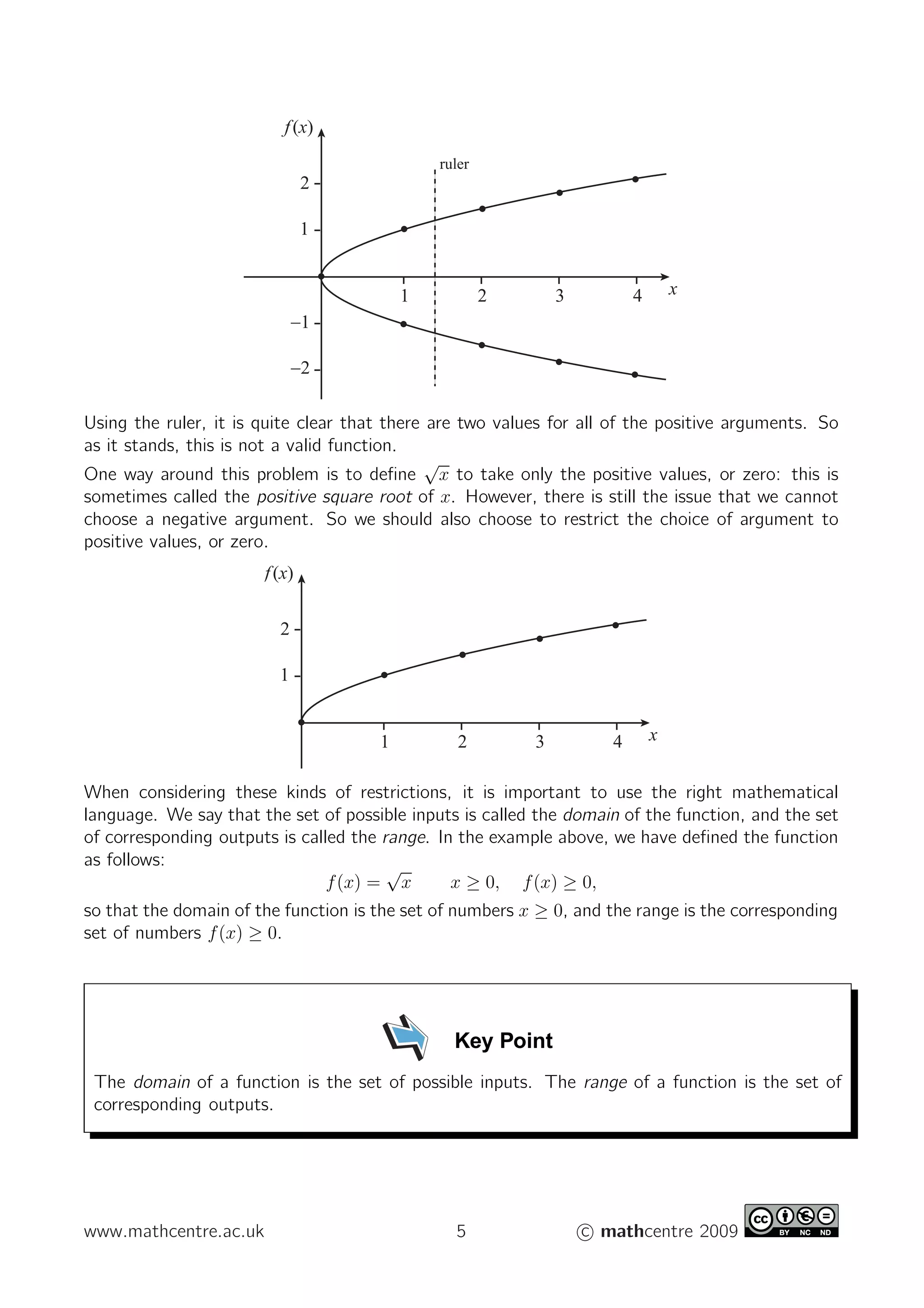
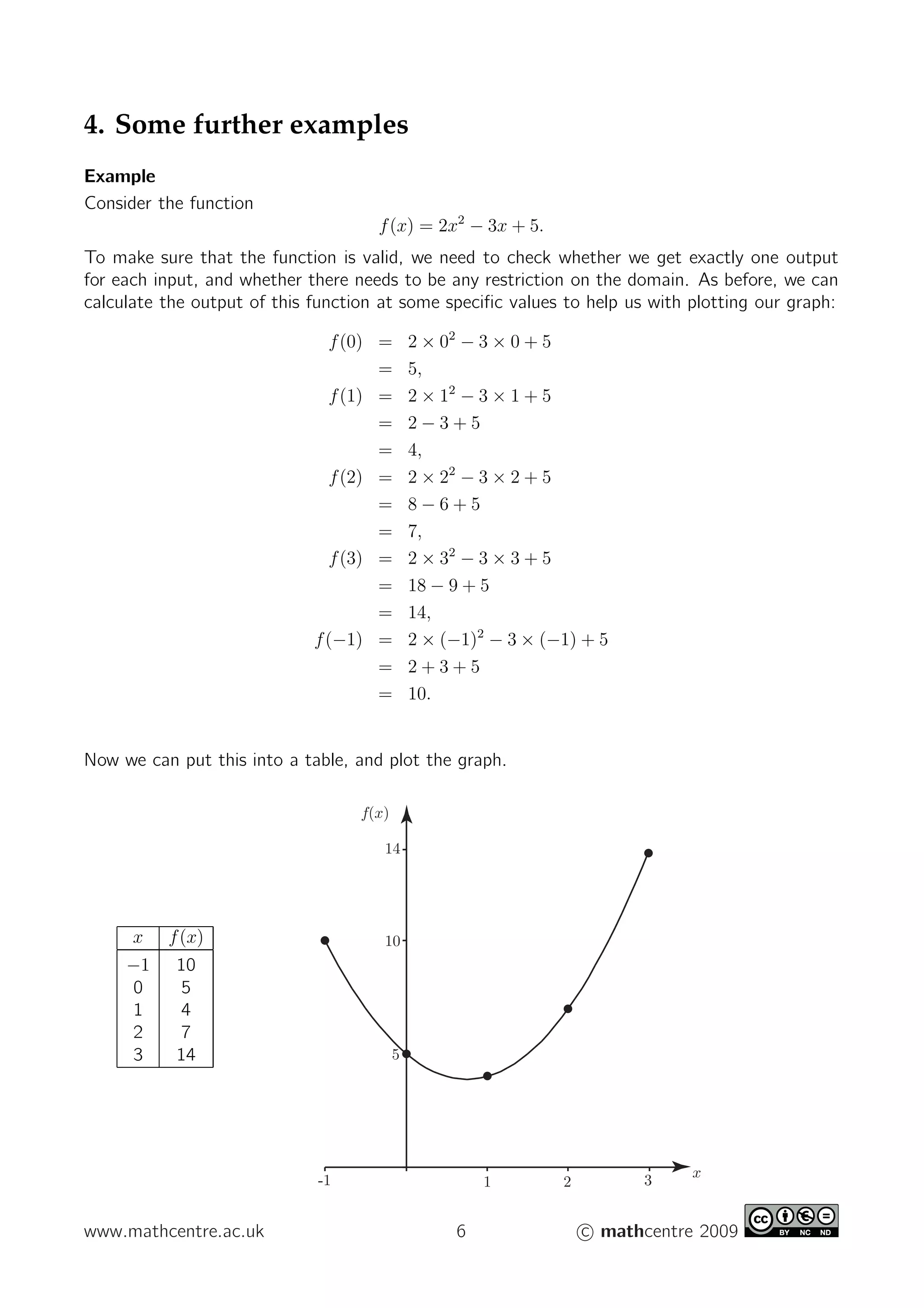
- A function is a rule that maps an input number (independent variable) to a unique output number (dependent variable).
- To determine if a rule describes a valid function, you can plot points from the rule on a graph and check that each input only maps to one output using a vertical ruler.
- For a rule to describe a valid function, its domain must be restricted if multiple outputs are possible for any single input. The domain is the set of possible inputs, and the range is the set of corresponding outputs.
Numerical method (curve fitting)
***TOPICS ARE****
Linear Regression
Multiple Linear Regression
Polynomial Regression
Example of Newton’s Interpolation Polynomial And example
Numerical method (curve fitting)
***TOPICS ARE****
Linear Regression
Multiple Linear Regression
Polynomial Regression
Example of Newton’s Interpolation Polynomial And example
This learner's module discusses or talks about the topic of Quadratic Functions. It also discusses what is Quadratic Functions. It also shows how to transform or rewrite the equation f(x)=ax2 + bx + c to f(x)= a(x-h)2 + k. It will also show the different characteristics of Quadratic Functions.
The Roman Empire A Historical Colossus.pdfkaushalkr1407
The Roman Empire, a vast and enduring power, stands as one of history's most remarkable civilizations, leaving an indelible imprint on the world. It emerged from the Roman Republic, transitioning into an imperial powerhouse under the leadership of Augustus Caesar in 27 BCE. This transformation marked the beginning of an era defined by unprecedented territorial expansion, architectural marvels, and profound cultural influence.
The empire's roots lie in the city of Rome, founded, according to legend, by Romulus in 753 BCE. Over centuries, Rome evolved from a small settlement to a formidable republic, characterized by a complex political system with elected officials and checks on power. However, internal strife, class conflicts, and military ambitions paved the way for the end of the Republic. Julius Caesar’s dictatorship and subsequent assassination in 44 BCE created a power vacuum, leading to a civil war. Octavian, later Augustus, emerged victorious, heralding the Roman Empire’s birth.
Under Augustus, the empire experienced the Pax Romana, a 200-year period of relative peace and stability. Augustus reformed the military, established efficient administrative systems, and initiated grand construction projects. The empire's borders expanded, encompassing territories from Britain to Egypt and from Spain to the Euphrates. Roman legions, renowned for their discipline and engineering prowess, secured and maintained these vast territories, building roads, fortifications, and cities that facilitated control and integration.
The Roman Empire’s society was hierarchical, with a rigid class system. At the top were the patricians, wealthy elites who held significant political power. Below them were the plebeians, free citizens with limited political influence, and the vast numbers of slaves who formed the backbone of the economy. The family unit was central, governed by the paterfamilias, the male head who held absolute authority.
Culturally, the Romans were eclectic, absorbing and adapting elements from the civilizations they encountered, particularly the Greeks. Roman art, literature, and philosophy reflected this synthesis, creating a rich cultural tapestry. Latin, the Roman language, became the lingua franca of the Western world, influencing numerous modern languages.
Roman architecture and engineering achievements were monumental. They perfected the arch, vault, and dome, constructing enduring structures like the Colosseum, Pantheon, and aqueducts. These engineering marvels not only showcased Roman ingenuity but also served practical purposes, from public entertainment to water supply.
2024.06.01 Introducing a competency framework for languag learning materials ...Sandy Millin
http://sandymillin.wordpress.com/iateflwebinar2024
Published classroom materials form the basis of syllabuses, drive teacher professional development, and have a potentially huge influence on learners, teachers and education systems. All teachers also create their own materials, whether a few sentences on a blackboard, a highly-structured fully-realised online course, or anything in between. Despite this, the knowledge and skills needed to create effective language learning materials are rarely part of teacher training, and are mostly learnt by trial and error.
Knowledge and skills frameworks, generally called competency frameworks, for ELT teachers, trainers and managers have existed for a few years now. However, until I created one for my MA dissertation, there wasn’t one drawing together what we need to know and do to be able to effectively produce language learning materials.
This webinar will introduce you to my framework, highlighting the key competencies I identified from my research. It will also show how anybody involved in language teaching (any language, not just English!), teacher training, managing schools or developing language learning materials can benefit from using the framework.
Ethnobotany and Ethnopharmacology:
Ethnobotany in herbal drug evaluation,
Impact of Ethnobotany in traditional medicine,
New development in herbals,
Bio-prospecting tools for drug discovery,
Role of Ethnopharmacology in drug evaluation,
Reverse Pharmacology.
Model Attribute Check Company Auto PropertyCeline George
In Odoo, the multi-company feature allows you to manage multiple companies within a single Odoo database instance. Each company can have its own configurations while still sharing common resources such as products, customers, and suppliers.
Unit 8 - Information and Communication Technology (Paper I).pdfThiyagu K
This slides describes the basic concepts of ICT, basics of Email, Emerging Technology and Digital Initiatives in Education. This presentations aligns with the UGC Paper I syllabus.
Palestine last event orientationfvgnh .pptxRaedMohamed3
An EFL lesson about the current events in Palestine. It is intended to be for intermediate students who wish to increase their listening skills through a short lesson in power point.
Read| The latest issue of The Challenger is here! We are thrilled to announce that our school paper has qualified for the NATIONAL SCHOOLS PRESS CONFERENCE (NSPC) 2024. Thank you for your unwavering support and trust. Dive into the stories that made us stand out!
We all have good and bad thoughts from time to time and situation to situation. We are bombarded daily with spiraling thoughts(both negative and positive) creating all-consuming feel , making us difficult to manage with associated suffering. Good thoughts are like our Mob Signal (Positive thought) amidst noise(negative thought) in the atmosphere. Negative thoughts like noise outweigh positive thoughts. These thoughts often create unwanted confusion, trouble, stress and frustration in our mind as well as chaos in our physical world. Negative thoughts are also known as “distorted thinking”.
Basic phrases for greeting and assisting costumers
Introduction to functions
1. Introduction to
functions
mc-TY-introfns-2009-1
A function is a rule which operates on one number to give another number. However, not every
rule describes a valid function. This unit explains how to see whether a given rule describes a
valid function, and introduces some of the mathematical terms associated with functions.
In order to master the techniques explained here it is vital that you undertake plenty of practice
exercises so that they become second nature.
After reading this text, and/or viewing the video tutorial on this topic, you should be able to:
• recognise when a rule describes a valid function,
• be able to plot the graph of a part of a function,
• find a suitable domain for a function, and find the corresponding range.
Contents
1. What is a function? 2
2. Plotting the graph of a function 3
3. When is a function valid? 4
4. Some further examples 6
www.mathcentre.ac.uk 1 c mathcentre 2009
2. 1. What is a function?
Here is a definition of a function.
A function is a rule which maps a number to another unique number.
In other words, if we start off with an input, and we apply the function, we get an output.
For example, we might have a function that added 3 to any number. So if we apply this function
to the number 2, we get the number 5. If we apply this function to the number 8, we get the
number 11. If we apply this function to the number x, we get the number x + 3.
We can show this mathematically by writing
f(x) = x + 3.
The number x that we use for the input of the function is called the argument of the function.
So if we choose an argument of 2, we get
f(2) = 2 + 3 = 5.
If we choose an argument of 8, we get
f(8) = 8 + 3 = 11.
If we choose an argument of −6, we get
f(−6) = −6 + 3 = −3.
If we choose an argument of z, we get
f(z) = z + 3.
If we choose an argument of x2
, we get
f(x2
) = x2
+ 3.
At first sight, it seems that we can pick any number we choose for the argument. However, that
is not the case, as we shall see later. But because we do have some choice in the number we
can pick, we call the argument the independent variable. The output of the function, e.g. f(x),
f(5), etc. depends upon the argument, and so this is called the dependent variable.
Key Point
A function is a rule that maps a number to another unique number.
The input to the function is called the independent variable, and is also called the argument of
the function. The output of the function is called the dependent variable.
www.mathcentre.ac.uk 2 c mathcentre 2009
3. 2. Plotting the graph of a function
If we have a function given by a formula, we can try to plot its graph. Suppose, for example,
that we have a function f defined by
f(x) = 3x2
− 4.
The argument of the function (the independent variable) is x, and the output (the dependent
variable) is 3x2
− 4. So we can calculate the output of the function for different arguments:
f(0) = 3 × 02
− 4 = −4
f(1) = 3 × 12
− 4 = −1
f(2) = 3 × 22
− 4 = 8
f(−1) = 3 × (−1)2
− 4 = −1
f(−2) = 3 × (−2)2
− 4 = 8.
We can put this information into a table to help us plot the graph of the function.
x f(x)
−2 8
−1 −1
0 −4
1 −1
2 8
f(x)
x−2 1 2−1
8
4
−4
We can use the graph of the function to find the output corresponding to a given argument. For
instance, if we have an argument of 2, we start on the horizontal axis at the point where x = 2,
and we follow the line up until we reach the graph. Then we follow the line across so that we
can read off the value of f(x) on the vertical axis. In this case, the value of f(x) is 8. Of course
we already know this, because x = 2 is one of the values in our table.
f(x)
x−2 1 2−1
8
4
−4
www.mathcentre.ac.uk 3 c mathcentre 2009
4. But we can also use the graph for values of x which are not in our table. If we have an argument
of 1.5, we follow the line up to the graph, and then across to the vertical axis. The result is a
number between 2 and 3.
f(x)
x−2 1 2−1
8
4
−4
If we want to calculate this number exactly, we can substitute 1.5 into the formula:
f(1.5) = 2.75
3. When is a function valid?
Our definition of a function says that it is a rule mapping a number to another unique number.
So we cannot have a function which gives two different outputs for the same argument. One
easy way to check this is from the graph of the function, by using a ruler. If the ruler is aligned
vertically, then it only ever crosses the graph once; no more and no less. This means that the
graph represents a valid function.
What happens if we try to define a function with more than one output for the same argument?
Let’s try an example. Suppose we try to define a function by saying that
f(x) =
√
x.
In the same way as before, we can produce a table of results to help us plot the graph of the
function:
f(0) = 0
f(1) = ±1
f(2) = ±1.4 to 1 d.p.
f(3) = ±1.7 to 1 d.p.
f(4) = ±2.
(If we try to use any negative arguments, we end up in trouble because we are trying to find
the square root of a negative number.) Plotting the results from the table, we get the following
graph.
www.mathcentre.ac.uk 4 c mathcentre 2009
5. f(x)
x2 3 41
2
−1
1
−2
ruler
Using the ruler, it is quite clear that there are two values for all of the positive arguments. So
as it stands, this is not a valid function.
One way around this problem is to define
√
x to take only the positive values, or zero: this is
sometimes called the positive square root of x. However, there is still the issue that we cannot
choose a negative argument. So we should also choose to restrict the choice of argument to
positive values, or zero.
f(x)
x2 3 41
2
1
When considering these kinds of restrictions, it is important to use the right mathematical
language. We say that the set of possible inputs is called the domain of the function, and the set
of corresponding outputs is called the range. In the example above, we have defined the function
as follows:
f(x) =
√
x x ≥ 0, f(x) ≥ 0,
so that the domain of the function is the set of numbers x ≥ 0, and the range is the corresponding
set of numbers f(x) ≥ 0.
Key Point
The domain of a function is the set of possible inputs. The range of a function is the set of
corresponding outputs.
www.mathcentre.ac.uk 5 c mathcentre 2009
6. 4. Some further examples
Example
Consider the function
f(x) = 2x2
− 3x + 5.
To make sure that the function is valid, we need to check whether we get exactly one output
for each input, and whether there needs to be any restriction on the domain. As before, we can
calculate the output of this function at some specific values to help us with plotting our graph:
f(0) = 2 × 02
− 3 × 0 + 5
= 5,
f(1) = 2 × 12
− 3 × 1 + 5
= 2 − 3 + 5
= 4,
f(2) = 2 × 22
− 3 × 2 + 5
= 8 − 6 + 5
= 7,
f(3) = 2 × 32
− 3 × 3 + 5
= 18 − 9 + 5
= 14,
f(−1) = 2 × (−1)2
− 3 × (−1) + 5
= 2 + 3 + 5
= 10.
Now we can put this into a table, and plot the graph.
x f(x)
−1 10
0 5
1 4
2 7
3 14
14
10
5
1 2 3-1
f(x)
x
www.mathcentre.ac.uk 6 c mathcentre 2009
7. A vertical ruler always crosses the graph once, and so the domain needs no restrictions, and
the function is valid. We can also see from the graph that the minimum output occurs when
x = 0.75, and that is when f(x) = 3.875. So the range of the function is f(x) ≥ 3.875.
Example
What about the function
f(x) =
1
x
?
As usual, the first step is to check some values.
f(1) = 1, f(2) = 1
2
, f(3) = 1
3
, f(4) = 1
4
,
f(−1) =
1
(−1)
= −1, f(−2) =
1
(−2)
= −1
2
,
f(−3) =
1
(−3)
= −1
3
, f(−4) =
1
(−4)
= −1
4
.
When we try to calculate f(0) we have a problem, because we cannot divide by zero. So we
have to restrict the domain to exclude x = 0.
f(x)
x−1−2 1 2 3 4−3−4
1
1
2
1
2
−
−1
Because of this problem when x = 0, we have to restrict the domain to make the function valid.
You can also see from the graph that there is no value of x where f(x) = 0, so zero is also
excluded from the range. The function is therefore defined by
f(x) = 1/x x = 0, f(x) = 0.
You might want to know what exactly is going on at this point when x = 0. One way to find
out is to look at what is happening very close to zero. So let’s try some positive values for the
argument getting closer and closer to zero, in order to see what happens:
f(1) = 1, f
1
2
=
1
1/2
= 2, f
1
10
=
1
1/10
= 10,
f
1
1,000
=
1
1/1,000
= 1,000, f
1
1,000,000
=
1
1/1,000,000
= 1,000,000 .
So you can see that as we approach zero from the right, the output approaches infinity.
www.mathcentre.ac.uk 7 c mathcentre 2009
8. Now let’s try some negative values for the argument, getting closer and closer to zero from the
left-hand side, in order to see what happens:
f(−1) =
1
(−1)
= −1, f −
1
2
=
1
(−1/2)
= −2, f −
1
10
=
1
(−1/10)
= −10,
f −
1
1,000
=
1
(−1/1,000)
= −1,000, f −
1
1,000,000
=
1
(−1/1,000,000)
= −1,000,000 .
You can see that as we approach zero from the left, the output approaches negative infinity. So
in this case, approaching zero from the left is very different from approaching it from the right.
Example
For our final example, take the function
f(x) =
1
(x − 2)2
.
As usual, we must calculate some values:
f(−2) =
1
(−2 − 2)2
= 1
16
f(−1) =
1
(−1 − 2)2
= 1
9
f(0) =
1
(0 − 2)2
= 1
4
f(1) =
1
(1 − 2)2
= 1
f(2) =
1
(2 − 2)2
= dividing by zero
f(3) =
1
(3 − 2)2
= 1
f(4) =
1
(4 − 2)2
= 1
4
f(5) =
1
(5 − 2)2
= 1
9
f(6) =
1
(6 − 2)2
= 1
16
.
Now we can construct a table, and plot the graph of the function.
x f(x)
−2 1
16
−1 1
9
0 1
4
1 1
2 dividing by zero
3 1
4 1
4
5 1
9
6 1
16
www.mathcentre.ac.uk 8 c mathcentre 2009
9. f(x)
x
1 2 3 4 5 6−1−2
1
1
4
3
4
1
2
The vertical line at x = 2 is called an asymptote; it is a line which is approached by the graph but
never reached. Although it is clear that we will have to omit x = 2 from the domain, this time the
situation is slightly different. You can see that at either side of x = 2, f(x) is approaching infinity.
You should also notice that we cannot have any negative values for f(x), or even f(x) = 0. So
we have to define our function as
f(x) =
1
(x − 2)2
x = 2, f(x) > 0.
Exercises
1. Consider the function
f(x) = 2x2
+ 5x − 3.
(a) Write down the argument of this function.
(b) Write down the dependent variable in terms of the argument.
(c) Use a table of values to help you plot the graph of the function.
(d) From your graph, estimate f(1.5).
(e) Use your function to calculate f(1.5) exactly.
(f) Write down the domain and range of the function.
(g) Re-write the function with argument y.
2. Consider the function
f(x) =
1
(x − 3)2
.
(a) Plot the graph of the function.
(b) Write down the domain and range of the function.
(c) Re-write the function with argument z.
(d) Use your graph to estimate f(1).
(e) Use the function to calculate f(1) exactly.
(f) Write down another function where x = 4 has to be omitted from the domain.
3. Consider the function
f(x) = 3
√
x.
(a) What assumptions must be made about the function to ensure validity?
(b) Plot the graph of the function.
www.mathcentre.ac.uk 9 c mathcentre 2009
10. (c) Write down the domain and range of the function.
(d) Calculate f(3).
(e) What happens if you try to calculate f(−2)?
4. Consider the function
f(x) =
1
x
.
(a) Plot the graph of the function.
(b) Write down the domain and range of the function.
(c) What happens to the output of the function as the argument approaches zero?
(d) Is approaching zero from the left different to approaching zero from the right? If yes, why?
(e) Calculate f(2), f(−10) and f(z3
).
5. In the following list, you should write down the domain and range for each function, and then
pair up functions that share the same domain and range.
f(x) = 2 sin x − 1
f(x) = x2
− 6x + 9
f(x) = 2e−x
f(x) = 4 − x2
f(x) = 2x − x2
+ 3
f(x) = 3e5x
f(x) = 2 cos 2x − 1
f(x) = 4x2
− 16x + 16
Answers
1.
(a) The argument is x.
(b) The dependent variable is 2x2
+ 5x − 3 in terms of x.
(c) An example of a table of values might be
x −4 −3 −2 −1 0 1 2
f(x) 9 0 −5 −6 −3 4 15
f(x)
x−4 2 4−2
8
4
−4
www.mathcentre.ac.uk 10 c mathcentre 2009
11. (d) Draw a line up from x = 1.5, and read off the value on the y-axis.
(e) f(1.5) = 9.
(f) Reading off from the graph, f(x) ≥ −6.125, and also −∞ < x < ∞.
(g) The function is f(y) = 2y2
+ 5y − 3 using an argument y.
www.mathcentre.ac.uk 11 c mathcentre 2009
12. 2.
(a)
f(x)
x2 4 6 8−2
6
4
2
(b) The domain is x = 3, the range is f(x) > 0.
(c) The function is f(z) =
1
(z − 3)2
using an argument z.
(d) Draw a line up from x = 1, and read off the value on the y-axis.
(e) f(1) =
1
(1 − 3)2
= 1
4
.
(f) One such function is f(x) =
1
(x − 4)2
, but there are many others.
3.
(a) We must assume that we take the positive square root, and that we take x ≥ 0.
(b)
f(x)
x5 10 15−5
10
5
(c) The domain is x ≥ 0, the range is f(x) ≥ 0.
(d) f(3) = 3
√
3 = 5.2 (to 1 d.p.).
(e) If you try to calculate f(−2), you will be attempting to find the square root of a negative
number. This has no real solutions.
www.mathcentre.ac.uk 12 c mathcentre 2009
13. 4.
(a)
f(x)
x
−2−4
2 4 6 8
4
−2
−4
2
−8 −6
(b) The domain is x = 0, the range is f(x) = 0.
(c) The output approaches ±∞.
(d) Approaching from the left is different to approaching from the right. Approaching from the
left, the output decreases rapidly to negative infinity. Approaching from the right, the output
increases rapidly to positive infinity.
(e) f(2) = 1
2
, f(−10) = − 1
10
, f(z3
) = 1/z3
.
5.
domain range
f(x) = 2 sin x − 1 −∞ < x < ∞ −3 ≤ f(x) ≤ 1
f(x) = x2
− 6x + 9 −∞ < x < ∞ f(x) ≥ 0
f(x) = 2e−x
−∞ < x < ∞ f(x) > 0
f(x) = 4 − x2
−∞ < x < ∞ f(x) ≤ 4
f(x) = 2x − x2
+ 3 −∞ < x < ∞ f(x) ≤ 4
f(x) = 3e5x
−∞ < x < ∞ f(x) > 0
f(x) = 2 cos 2x − 1 −∞ < x < ∞ −3 ≤ f(x) ≤ 1
f(x) = 4x2
− 16x + 16 −∞ < x < ∞ f(x) ≥ 0
So the pairs are
f(x) = 2 sin(x) − 1 and f(x) = 2 cos 2x − 1 ,
f(x) = x2
− 6x + 9 and f(x) = 4x2
− 16x + 16 ,
f(x) = 2e−x
and f(x) = 3e5x
,
f(x) = 4 − x2
and f(x) = 2x − x2
+ 3 .
www.mathcentre.ac.uk 13 c mathcentre 2009