Download as PDF, PPTX
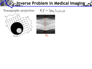
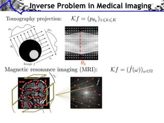

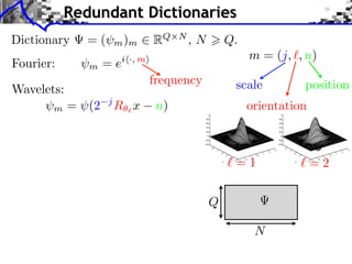
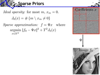
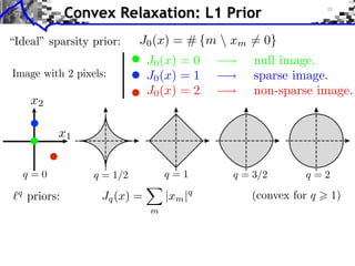
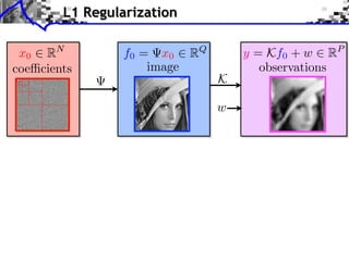
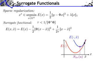
![Noiseless Sparse Regularization
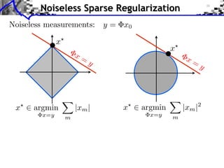
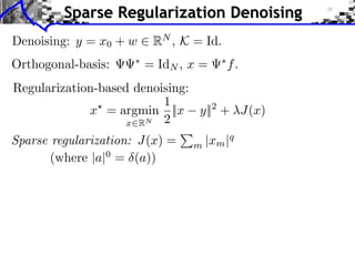
Noiseless measurements: y = x0
x
x
x= x=
y y
x argmin |xm | x argmin |xm |2
x=y m x=y m
Convex linear program.
Interior points, cf. [Chen, Donoho, Saunders] “basis pursuit”.
Douglas-Rachford splitting, see [Combettes, Pesquet].](https://image.slidesharecdn.com/course-signal-inverse-pbm-sparse-121213053017-phpapp01/85/Signal-Processing-Course-Sparse-Regularization-of-Inverse-Problems-37-320.jpg)
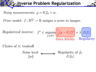
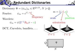
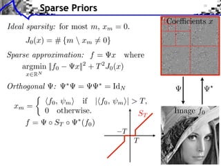
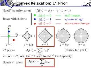
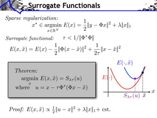
![Noisy Sparse Regularization
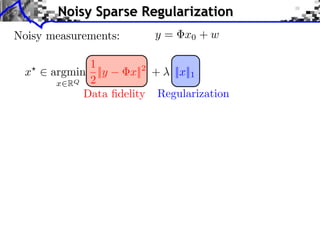
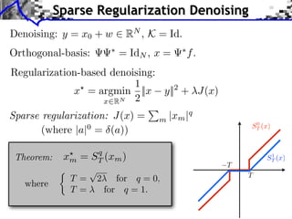
Noisy measurements: y = x0 + w
1
x argmin ||y x||2 + ||x||1
x RQ 2 Equivalence
Data fidelity Regularization
x argmin ||x||1
|| x y||
|
x=
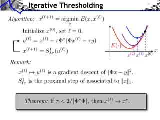
Algorithms: x y|
Iterative soft thresholding
Forward-backward splitting
see [Daubechies et al], [Pesquet et al], etc
Nesterov multi-steps schemes.](https://image.slidesharecdn.com/course-signal-inverse-pbm-sparse-121213053017-phpapp01/85/Signal-Processing-Course-Sparse-Regularization-of-Inverse-Problems-40-320.jpg)
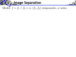
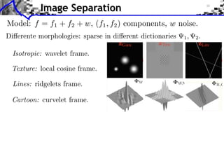
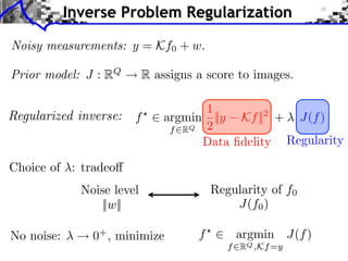
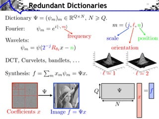
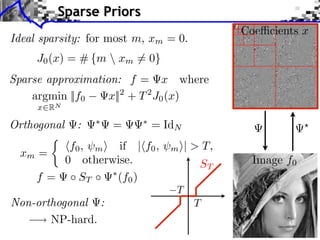
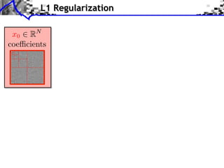
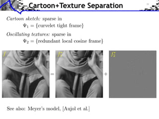
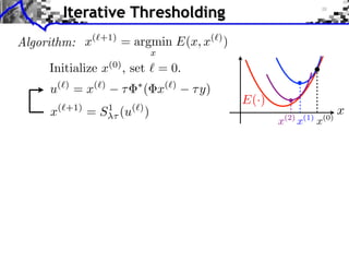
![Image Separation
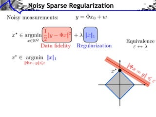
Model: f = f1 + f2 + w, (f1 , f2 ) components, w noise.
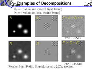
Union dictionary: =[ 1, 2] RQ (N1 +N2 )
Recovered component: fi = i xi .
1
(x1 , x2 ) argmin ||f x||2 + ||x||1
x=(x1 ,x2 ) RN 2](https://image.slidesharecdn.com/course-signal-inverse-pbm-sparse-121213053017-phpapp01/85/Signal-Processing-Course-Sparse-Regularization-of-Inverse-Problems-49-320.jpg)
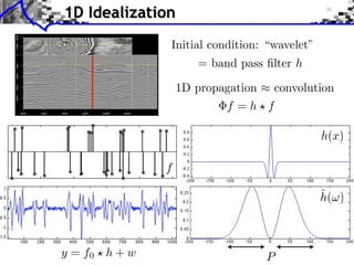
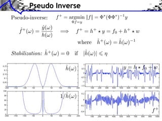
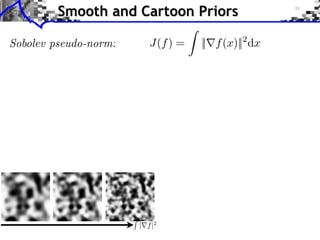
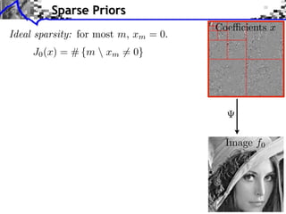
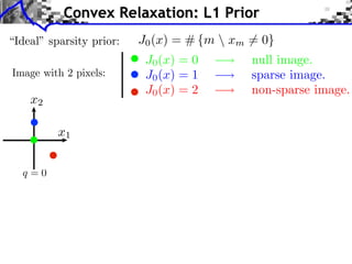
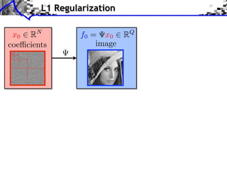
![Sparse Spikes Deconvolution
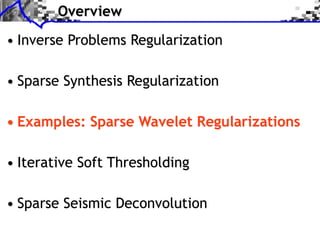
f with small ||f ||0 y=f h+w
Sparsity basis: Diracs ⇥m [x] = [x m]
1
f = argmin ||f ⇥ h y||2 + |f [m]|.
f RN 2 m](https://image.slidesharecdn.com/course-signal-inverse-pbm-sparse-121213053017-phpapp01/85/Signal-Processing-Course-Sparse-Regularization-of-Inverse-Problems-64-320.jpg)
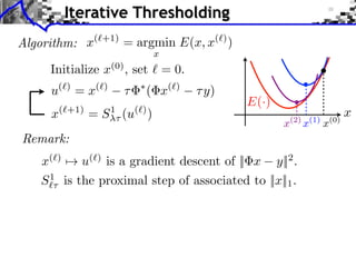
![Sparse Spikes Deconvolution
f with small ||f ||0 y=f h+w
Sparsity basis: Diracs ⇥m [x] = [x m]
1
f = argmin ||f ⇥ h y||2 + |f [m]|.
f RN 2 m
Algorithm: < 2/|| ˆ
|| = 2/max |h(⇥)|2
˜
• Inversion: f (k) = f (k) h ⇥ (h ⇥ f (k) y).
˜
f (k+1) [m] = S 1⇥ (f (k) [m])](https://image.slidesharecdn.com/course-signal-inverse-pbm-sparse-121213053017-phpapp01/85/Signal-Processing-Course-Sparse-Regularization-of-Inverse-Problems-65-320.jpg)
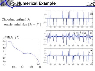
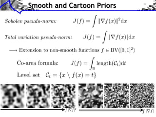
![Convergence Study
Sparse deconvolution:f = argmin E(f ).
f RN
1
Energy: E(f ) = ||h ⇥ f y||2 + |f [m]|.
2 m
Not strictly convex = no convergence speed.
log10 (E(f (k) )/E(f ) 1) log10 (||f (k) f ||/||f0 ||)
k k](https://image.slidesharecdn.com/course-signal-inverse-pbm-sparse-121213053017-phpapp01/85/Signal-Processing-Course-Sparse-Regularization-of-Inverse-Problems-67-320.jpg)
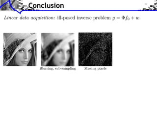
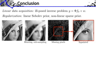
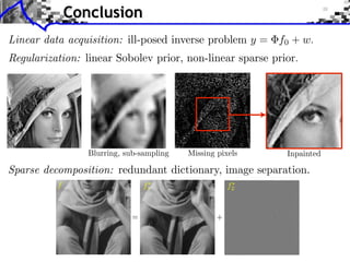

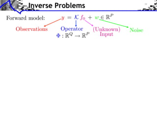
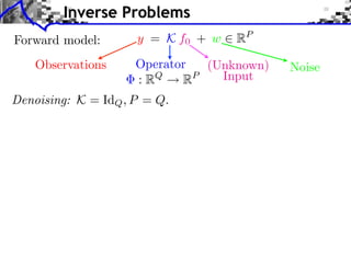
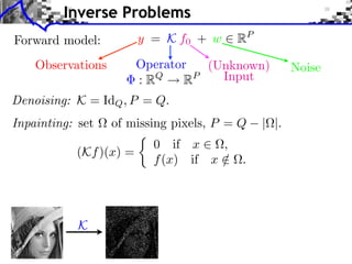
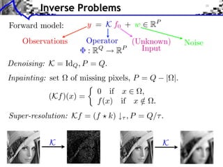
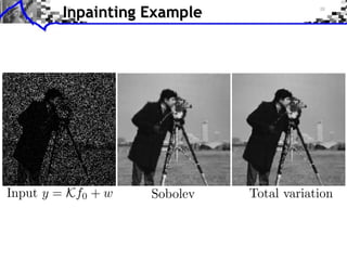
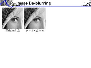
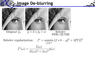
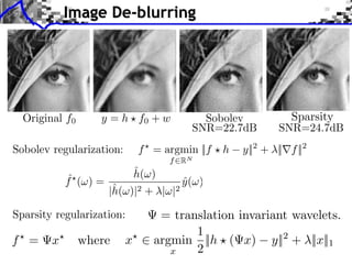
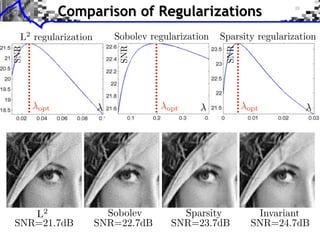
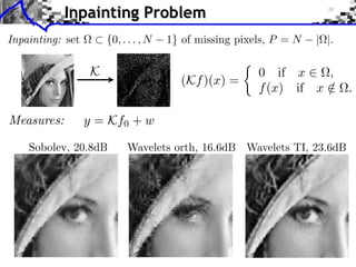
The document discusses sparse regularization for inverse problems. It describes how sparse regularization can be used for tasks like denoising, inpainting, and image separation by posing them as optimization problems that minimize data fidelity and an L1 sparsity prior on the coefficients. Iterative soft thresholding is presented as an algorithm for solving the noisy sparse regularization problem. Examples are given of how sparse wavelet regularization can outperform other regularizers like Sobolev for tasks like image deblurring.