This document discusses regularization techniques for inverse problems. It introduces variational priors like Sobolev and total variation to regularize inverse problems. Gradient descent and proximal gradient methods are presented to minimize regularization functionals for problems like denoising. Conjugate gradient and projected gradient descent are discussed for solving the regularized inverse problems. Total variation priors are shown to better recover edges compared to Sobolev priors. Non-smooth optimization methods may be needed to handle non-differentiable total variation functionals.

1. Inverse Problems
Regularization
www.numerical-tours.com
Gabriel Peyré

2. Overview
• Variational Priors
• Gradient Descent and PDE’s
• Inverse Problems Regularization

3. J(f) = ||f||2
W 1,2 =
Z
R2
||rf(x)||dxSobolev semi-norm:
Smooth and Cartoon Priors
| f|2

4. J(f) = ||f||2
W 1,2 =
Z
R2
||rf(x)||dxSobolev semi-norm:
Total variation semi-norm: J(f) = ||f||TV =
Z
R2
||rf(x)||dx
Smooth and Cartoon Priors
| f|| f|2

5. J(f) = ||f||2
W 1,2 =
Z
R2
||rf(x)||dxSobolev semi-norm:
Total variation semi-norm: J(f) = ||f||TV =
Z
R2
||rf(x)||dx
Smooth and Cartoon Priors
| f|| f|2

6. Natural Image Priors

7. Discrete Priors

8. Discrete Priors

9. Discrete Differential Operators

10. Discrete Differential Operators

11. Laplacian Operator

12. Laplacian Operator

13. Function: ˜f : x 2 R2
7! f(x) 2 R
˜f(x + ") = ˜f(x) + hrf(x), "iR2 + O(||"||2
R2 )
r ˜f(x) = (@1
˜f(x), @2
˜f(x)) 2 R2
Gradient: Images vs. Functionals

14. Function: ˜f : x 2 R2
7! f(x) 2 R
Discrete image: f 2 RN
, N = n2
f[i1, i2] = ˜f(i1/n, i2/n) rf[i] ⇡ r ˜f(i/n)
˜f(x + ") = ˜f(x) + hrf(x), "iR2 + O(||"||2
R2 )
r ˜f(x) = (@1
˜f(x), @2
˜f(x)) 2 R2
Gradient: Images vs. Functionals

15. Function: ˜f : x 2 R2
7! f(x) 2 R
Discrete image: f 2 RN
, N = n2
f[i1, i2] = ˜f(i1/n, i2/n)
Functional: J : f 2 RN
7! J(f) 2 R
J(f + ⌘) = J(f) + hrJ(f), ⌘iRN + O(||⌘||2
RN )
rf[i] ⇡ r ˜f(i/n)
˜f(x + ") = ˜f(x) + hrf(x), "iR2 + O(||"||2
R2 )
r ˜f(x) = (@1
˜f(x), @2
˜f(x)) 2 R2
rJ : RN
7! RN
Gradient: Images vs. Functionals

16. Function: ˜f : x 2 R2
7! f(x) 2 R
Discrete image: f 2 RN
, N = n2
f[i1, i2] = ˜f(i1/n, i2/n)
Functional: J : f 2 RN
7! J(f) 2 R
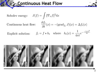
Sobolev:
rJ(f) = (r⇤
r)f = f
J(f) =
1
2
||rf||2
J(f + ⌘) = J(f) + hrJ(f), ⌘iRN + O(||⌘||2
RN )
rf[i] ⇡ r ˜f(i/n)
˜f(x + ") = ˜f(x) + hrf(x), "iR2 + O(||"||2
R2 )
r ˜f(x) = (@1
˜f(x), @2
˜f(x)) 2 R2
rJ : RN
7! RN
Gradient: Images vs. Functionals

17. rJ(f) = div
✓
rf
||rf||
◆
If 8 n, rf[n] 6= 0,
If 9n, rf[n] = 0, J not di↵erentiable at f.
Total Variation Gradient
||rf||
rJ(f)

18. rJ(f) = div
✓
rf
||rf||
◆
If 8 n, rf[n] 6= 0,
Sub-di↵erential:
If 9n, rf[n] = 0, J not di↵erentiable at f.
Cu = ↵ 2 R2⇥N
(u[n] = 0) ) (↵[n] = u[n]/||u[n]||)
@J(f) = { div(↵) ; ||↵[n]|| 6 1 and ↵ 2 Crf }
Total Variation Gradient
||rf||
rJ(f)

19. −10 −8 −6 −4 −2 0 2 4 6 8 10
−2
0
2
4
6
8
10
12
−10 −8 −6 −4 −2 0 2 4 6 8 10
−2
0
2
4
6
8
10
12
p
x2 + "2
|x|
Regularized Total Variation
||u||" =
p
||u||2 + "2 J"(f) =
P
n ||rf[n]||"

20. −10 −8 −6 −4 −2 0 2 4 6 8 10
−2
0
2
4
6
8
10
12
−10 −8 −6 −4 −2 0 2 4 6 8 10
−2
0
2
4
6
8
10
12
rJ"(f) = div
✓
rf
||rf||"
◆
p
x2 + "2
|x|
rJ" ⇠ /" when " ! +1
Regularized Total Variation
||u||" =
p
||u||2 + "2 J"(f) =
P
n ||rf[n]||"
rJ"(f)

21. Overview
• Variational Priors
• Gradient Descent and PDE’s
• Inverse Problems Regularization

22. f(k+1)
= f(k)
⌧krJ(f(k)
) f(0)
is given.
Gradient Descent

23. and 0 < ⌧ < 2/L, then f(k) k!+1
! f?
a solution of min
f
J(f).
If f is convex, C1
, rf is L-Lipschitz,Theorem:
f(k+1)
= f(k)
⌧krJ(f(k)
) f(0)
is given.
Gradient Descent

24. and 0 < ⌧ < 2/L, then f(k) k!+1
! f?
a solution of min
f
J(f).
If f is convex, C1
, rf is L-Lipschitz,Theorem:
f(k+1)
= f(k)
⌧krJ(f(k)
) f(0)
is given.
Optimal step size: ⌧k = argmin
⌧2R+
J(f(k)
⌧rJ(f(k)
))
Proposition: One has
hrJ(f(k+1)
), rJ(f(k)
)i = 0
Gradient Descent

25. Gradient Flows and PDE’s
f(k+1)
f(k)
⌧
= rJ(f(k)
)Fixed step size ⌧k = ⌧:

26. Gradient Flows and PDE’s
f(k+1)
f(k)
⌧
= rJ(f(k)
)Fixed step size ⌧k = ⌧:
Denote ft = f(k)
for t = k⌧, one obtains formally as ⌧ ! 0:
8 t > 0,
@ft
@t
= rJ(ft) and f0 = f(0)

27. J(f) =
R
||rf(x)||dxSobolev flow:
@ft
@t
= ftHeat equation:
Explicit solution:
Gradient Flows and PDE’s
f(k+1)
f(k)
⌧
= rJ(f(k)
)Fixed step size ⌧k = ⌧:
Denote ft = f(k)
for t = k⌧, one obtains formally as ⌧ ! 0:
8 t > 0,
@ft
@t
= rJ(ft) and f0 = f(0)

28. Total Variation Flow

29. @ft
@t
= rJ(ft)
Noisy observations: y = f + w, w ⇠ N(0, IdN ).
and ft=0 = y
Application: Denoising

30. Optimal choice of t: minimize ||ft f||
! not accessible in practice.
SNR(ft, f) = 20 log10
✓
||f ft||
||f||
◆
Optimal Parameter Selection
t t

31. Overview
• Variational Priors
• Gradient Descent and PDE’s
• Inverse Problems Regularization

32. Inverse Problems

33. Inverse Problems

34. Inverse Problems

35. Inverse Problems

36. Inverse Problems

37. Inverse Problem Regularization

38. Inverse Problem Regularization

39. Inverse Problem Regularization

40. Sobolev prior: J(f) = 1
2 ||rf||2
f?
= argmin
f2RN
E(f) = ||y f||2
+ ||rf||2
(assuming 1 /2 ker( ))
Sobolev Regularization

41. Sobolev prior: J(f) = 1
2 ||rf||2
f?
= argmin
f2RN
E(f) = ||y f||2
+ ||rf||2
rE(f?
) = 0 () ( ⇤
)f?
= ⇤
yProposition:
! Large scale linear system.
(assuming 1 /2 ker( ))
Sobolev Regularization

42. Sobolev prior: J(f) = 1
2 ||rf||2
f?
= argmin
f2RN
E(f) = ||y f||2
+ ||rf||2
rE(f?
) = 0 () ( ⇤
)f?
= ⇤
yProposition:
! Large scale linear system.
Gradient descent:
(assuming 1 /2 ker( ))
where ||A|| = max(A)
! Slow convergence.
Sobolev Regularization
Convergence: ⇥ < 2/||⇥ ⇥ ||

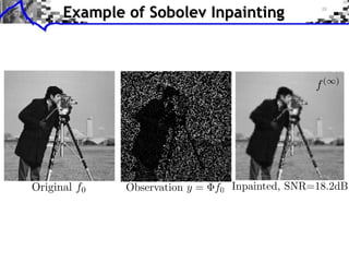
43. Mask M, = diagi(1i2M )
Example: InpaintingFigure 3 shows iterations of the algorithm 1 to solve the inpainting problem
on a smooth image using a manifold prior with 2D linear patches, as defined in
16. This manifold together with the overlapping of the patches allow a smooth
interpolation of the missing pixels.
Measurements y Iter. #1 Iter. #3 Iter. #50
Fig. 3. Iterations of the inpainting algorithm on an uniformly regular image.
5 Manifold of Step Discontinuities
In order to introduce some non-linearity in the manifold M, one needs to go
log10(||f(k)
f( )
||/||f0||)
k k
E(f(k)
)
M
( f)[i] =
⇢
0 if i 2 M,
f[i] otherwise.

44. Symmetric linear system:
Conjugate Gradient
Ax = b () min
x2Rn
E(x) =
1
2
hAx, xi hx, bi

45. Symmetric linear system:
x(k+1)
= argmin E(x)
s.t. x x(k)
2 span(rE(x(0)
), . . . , rE(x(k)
))
Intuition:
Conjugate Gradient
Ax = b () min
x2Rn
E(x) =
1
2
hAx, xi hx, bi
Proposition: 8 ` < k, hrE(xk
), rE(x`
)i = 0

46. Symmetric linear system:
Initialization: x(0)
2 RN
, r(0)
= b Ax(0)
, p(0)
= r(0)
r(k)
=
hrE(x(k)
), d(k)
i
hAd(k), d(k)i
d(k)
= rE(x(k)
) +
||v(k)
||
||v(k 1)||
d(k 1)
v(k)
= rE(x(k)
) = Ax(k)
b
x(k+1)
= x(k)
r(k)
d(k)
Iterations:
x(k+1)
= argmin E(x)
s.t. x x(k)
2 span(rE(x(0)
), . . . , rE(x(k)
))
Intuition:
Conjugate Gradient
Ax = b () min
x2Rn
E(x) =
1
2
hAx, xi hx, bi
Proposition: 8 ` < k, hrE(xk
), rE(x`
)i = 0

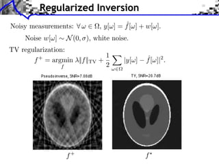
47. TV" regularization: (assuming 1 /2 ker( ))
f?
= argmin
f2RN
E(f) =
1
2
|| f y|| + J"
(f)
Total Variation Regularization
||u||" =
p
||u||2 + "2 J"(f) =
P
n ||rf[n]||"

48. TV" regularization: (assuming 1 /2 ker( ))
f(k+1)
= f(k)
⌧krE(f(k)
)
rE(f) = ⇤
( f y) + rJ"(f)
rJ"(f) = div
✓
rf
||rf||"
◆
Convergence: requires ⌧ ⇠ ".
Gradient descent:
f?
= argmin
f2RN
E(f) =
1
2
|| f y|| + J"
(f)
Total Variation Regularization
||u||" =
p
||u||2 + "2 J"(f) =
P
n ||rf[n]||"

49. TV" regularization: (assuming 1 /2 ker( ))
f(k+1)
= f(k)
⌧krE(f(k)
)
rE(f) = ⇤
( f y) + rJ"(f)
rJ"(f) = div
✓
rf
||rf||"
◆
Convergence: requires ⌧ ⇠ ".
Gradient descent:
f?
= argmin
f2RN
E(f) =
1
2
|| f y|| + J"
(f)
Newton descent:
f(k+1)
= f(k)
H 1
k rE(f(k)
) where Hk = @2
E"(f(k)
)
Total Variation Regularization
||u||" =
p
||u||2 + "2 J"(f) =
P
n ||rf[n]||"

50. k
Large" TV vs. Sobolev ConvergeSmall"

51. Observations y Sobolev Total variation
Inpainting: Sobolev vs. TV

52. Noiseless problem: f?
2 argmin
f
J"
(f) s.t. f 2 H
Contraint: H = {f ; f = y}.
f(k+1)
= ProjH
⇣
f(k)
⌧krJ"(f(k)
)
⌘
ProjH(f) = argmin
g=y
||g f||2
= f + ⇤
( ⇤
) 1
(y f)
Inpainting: ProjH(f)[i] =
⇢
f[i] if i 2 M,
y[i] otherwise.
Projected gradient descent:
f(k) k!+1
! f?
a solution of (?).
(?)
Projected Gradient Descent
Proposition: If rJ" is L-Lipschitz and 0 < ⌧k < 2/L,

53. TV
Priors: Non-quadratic
better edge recovery.
=)
Conclusion
Sobolev

54. TV
Priors: Non-quadratic
better edge recovery.
=)
Optimization
Variational regularization:
()
– Gradient descent. – Newton.
– Projected gradient. – Conjugate gradient.
Non-smooth optimization ?
Conclusion
Sobolev