Download as PDF, PPTX


![Noiseless Sparse Regularization
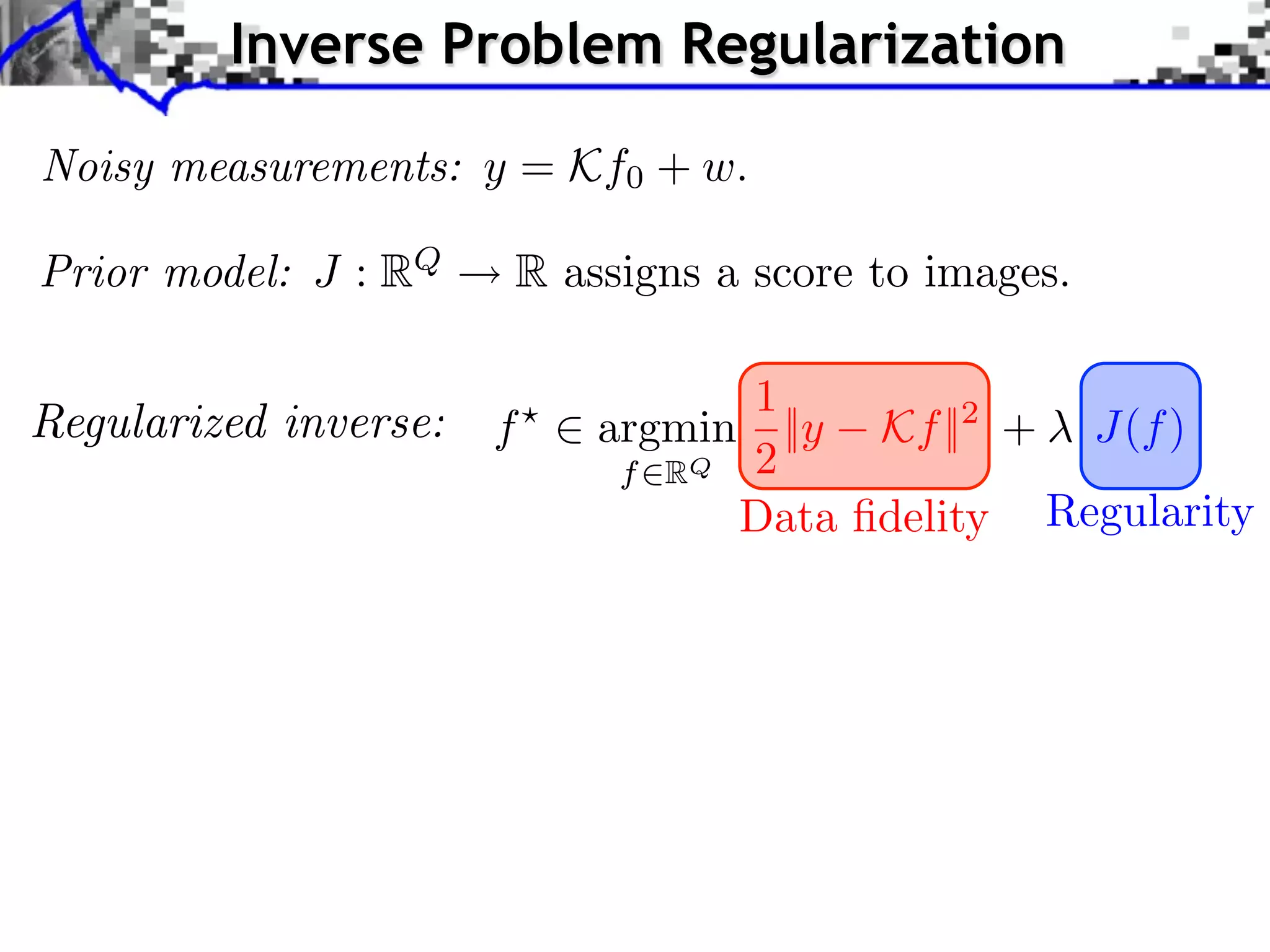
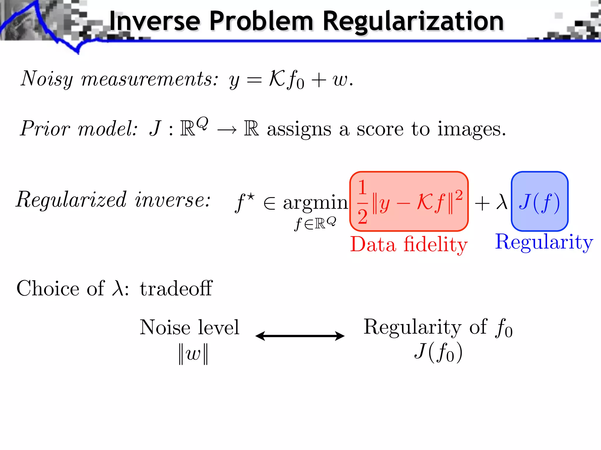
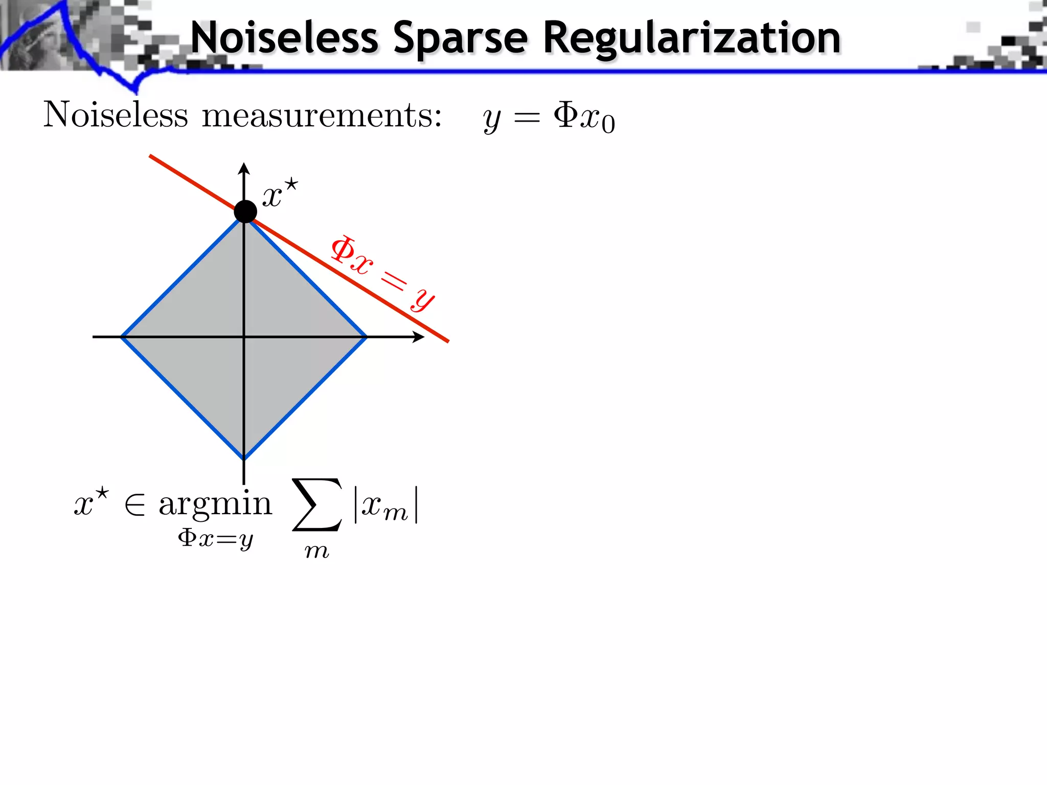
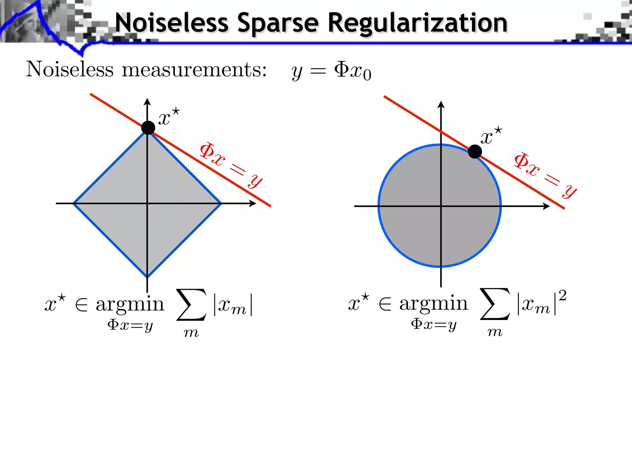
Noiseless measurements: y = x0
x
x
x= x=
y y
x argmin |xm | x argmin |xm |2
x=y m x=y m
Convex linear program.
Interior points, cf. [Chen, Donoho, Saunders] “basis pursuit”.
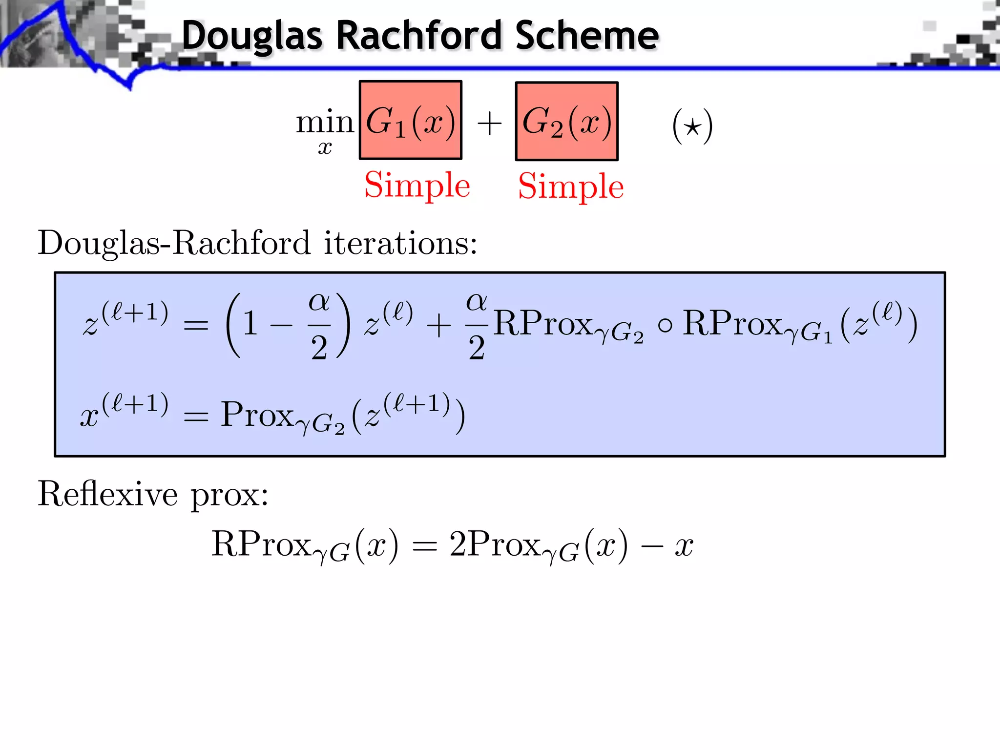
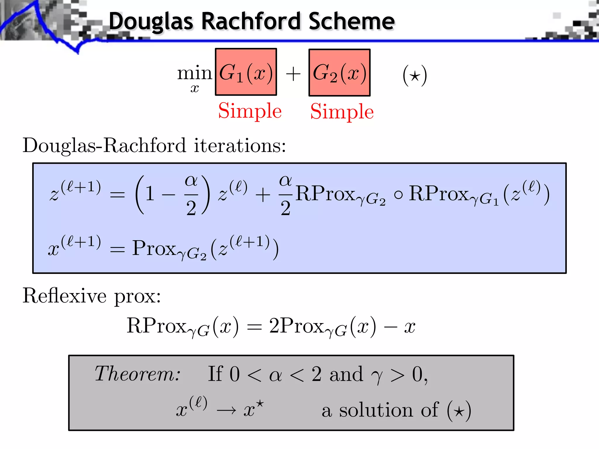
Douglas-Rachford splitting, see [Combettes, Pesquet].](https://image.slidesharecdn.com/2012-07-10-centrale-121213050709-phpapp02/75/Sparsity-and-Compressed-Sensing-37-2048.jpg)
![Noisy Sparse Regularization
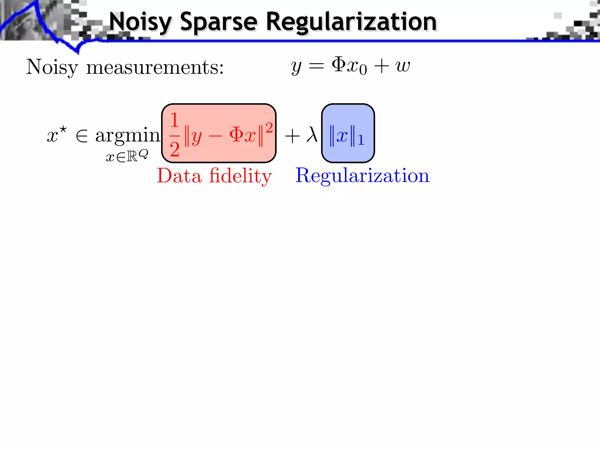
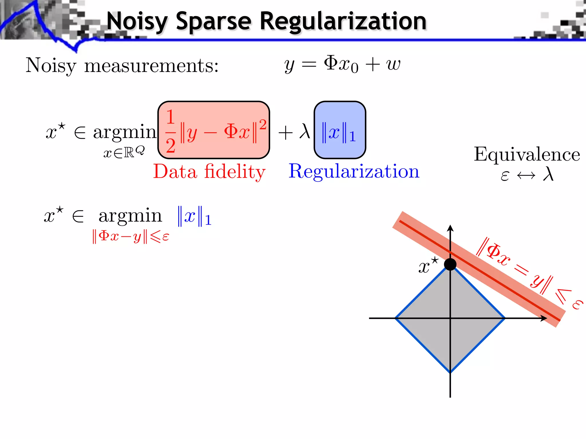
Noisy measurements: y = x0 + w
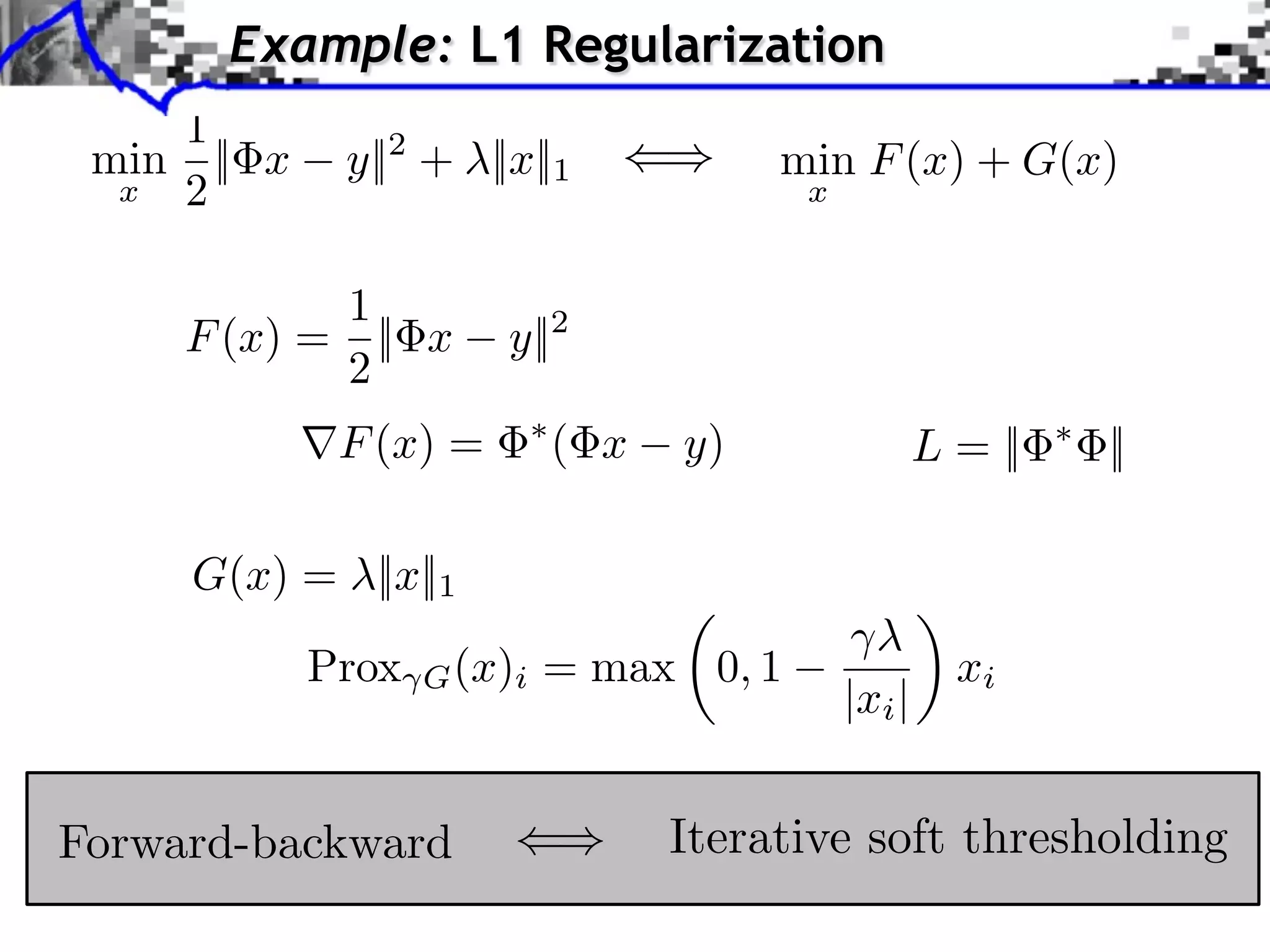
1
x argmin ||y x||2 + ||x||1
x RQ 2 Equivalence
Data fidelity Regularization
x argmin ||x||1
|| x y||
|
x=
Algorithms: x y|
Iterative soft thresholding
Forward-backward splitting
see [Daubechies et al], [Pesquet et al], etc
Nesterov multi-steps schemes.](https://image.slidesharecdn.com/2012-07-10-centrale-121213050709-phpapp02/75/Sparsity-and-Compressed-Sensing-40-2048.jpg)
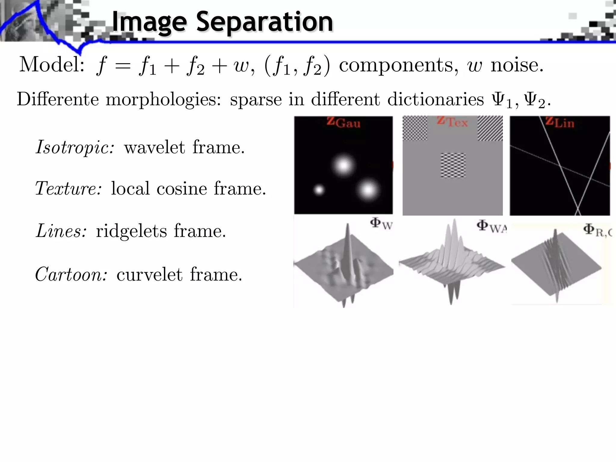
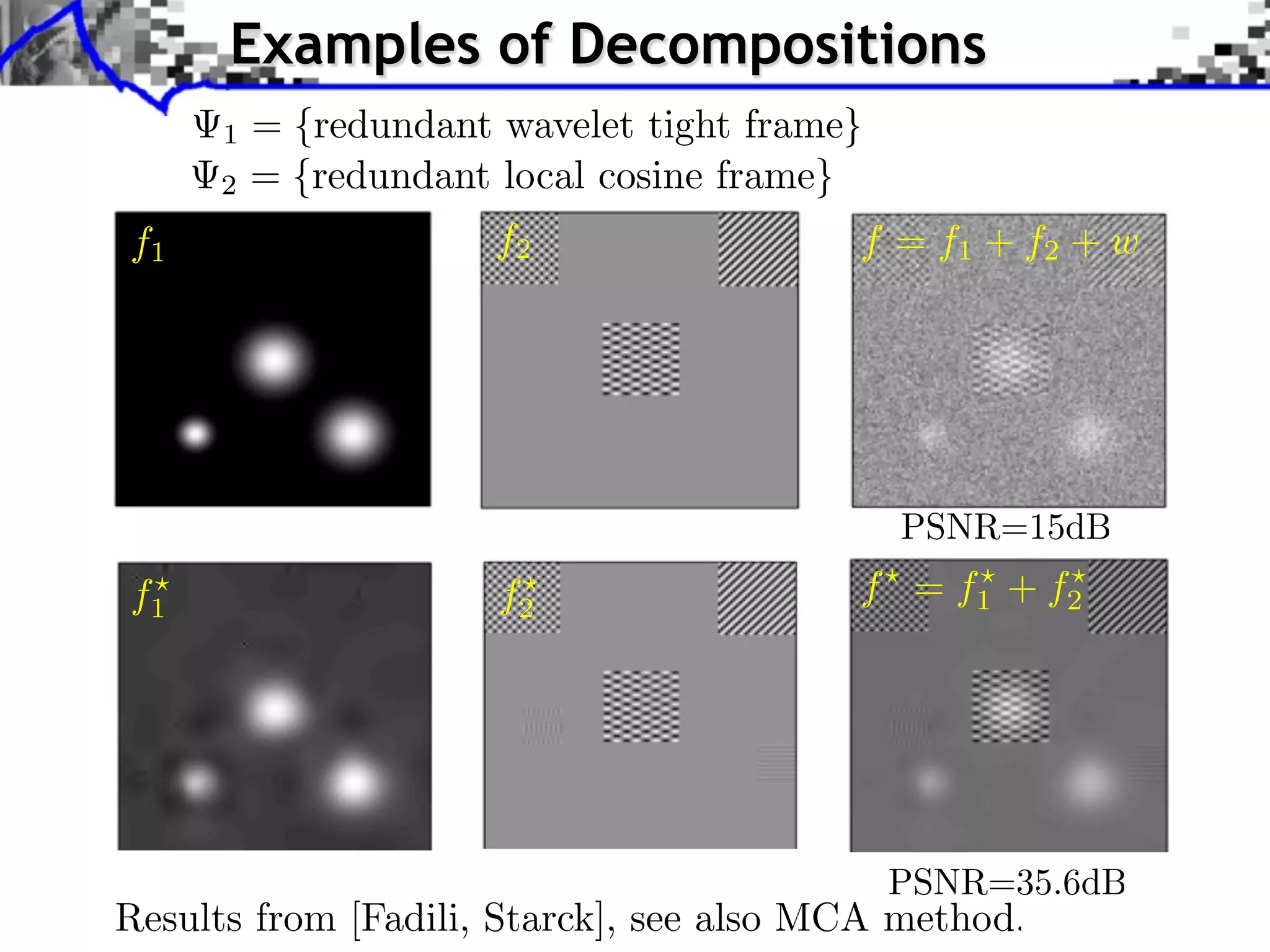
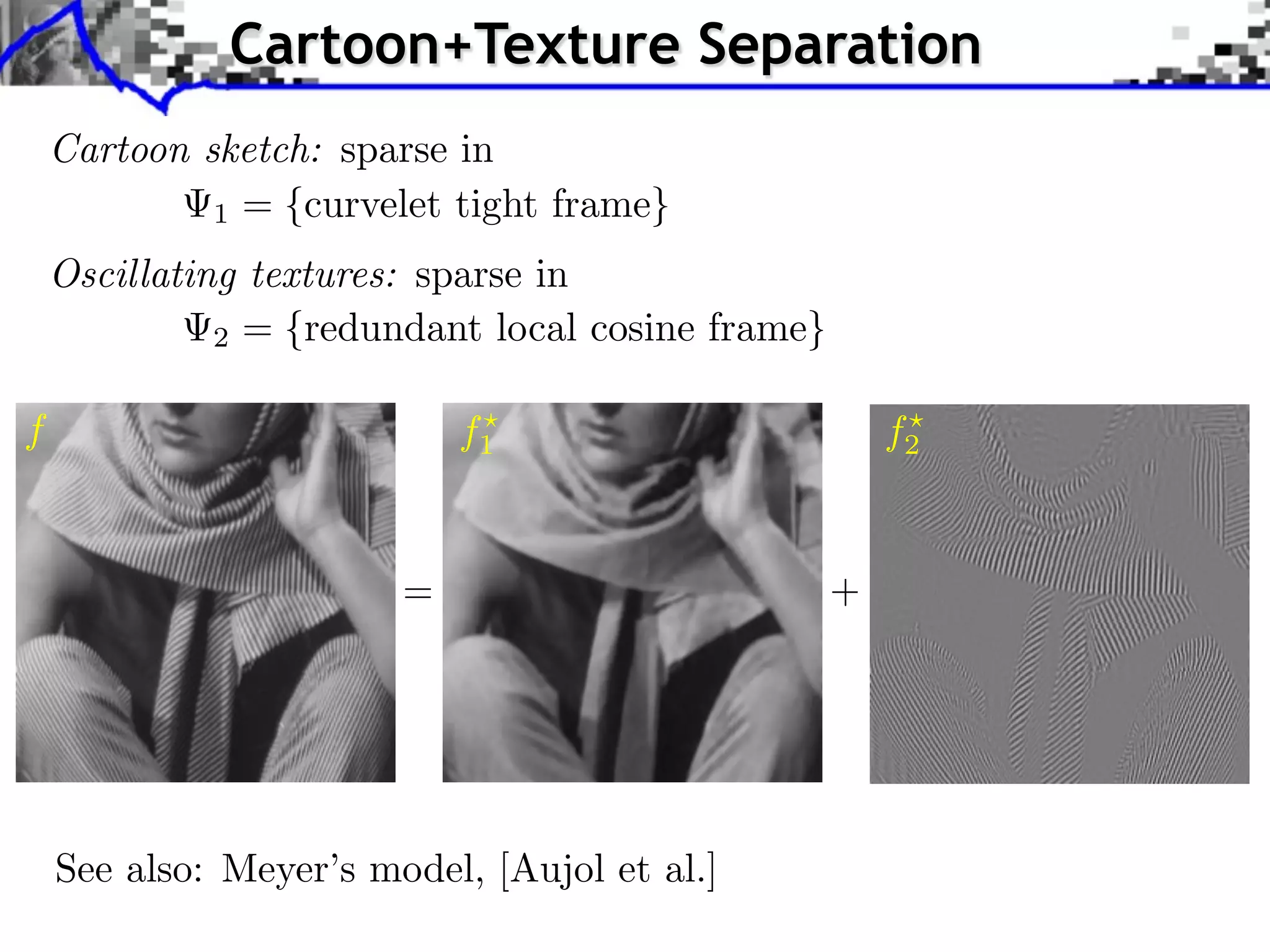
![Image Separation
Model: f = f1 + f2 + w, (f1 , f2 ) components, w noise.
Union dictionary: =[ 1, 2] RQ (N1 +N2 )
Recovered component: fi = i xi .
1
(x1 , x2 ) argmin ||f x||2 + ||x||1
x=(x1 ,x2 ) RN 2](https://image.slidesharecdn.com/2012-07-10-centrale-121213050709-phpapp02/75/Sparsity-and-Compressed-Sensing-47-2048.jpg)
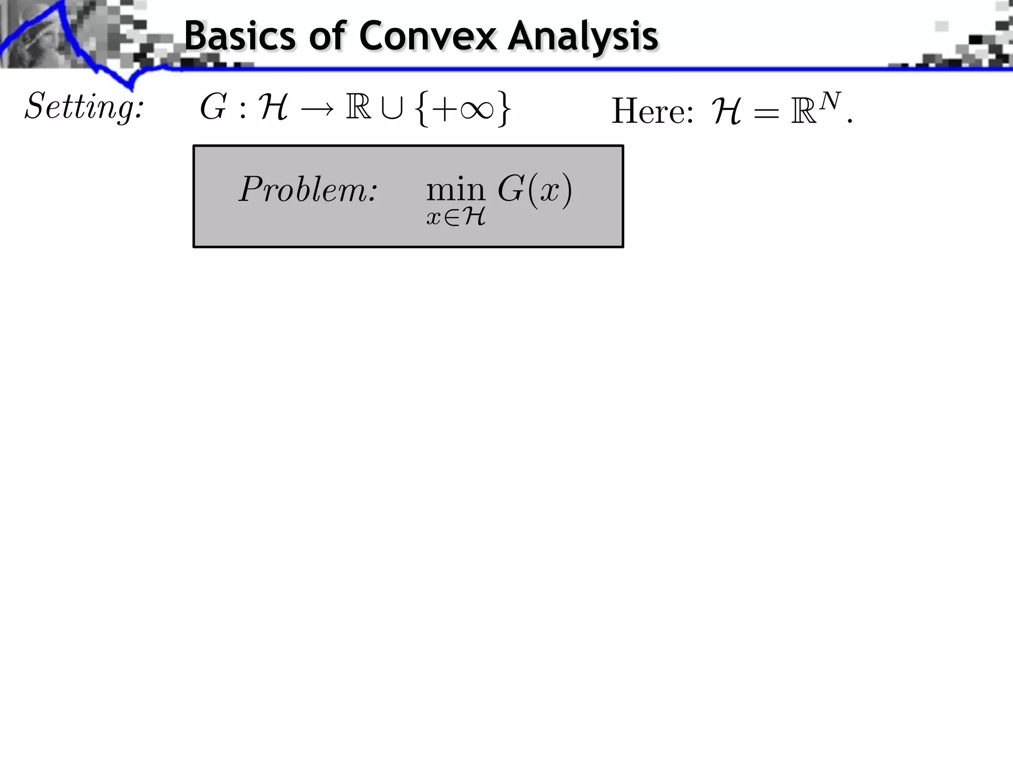
![Basics of Convex Analysis
Setting: G:H R ⇤ {+⇥} Here: H = RN .
Problem: min G(x)
x H
Convex: t [0, 1]
x y
G(tx + (1 t)y) tG(x) + (1 t)G(y)](https://image.slidesharecdn.com/2012-07-10-centrale-121213050709-phpapp02/75/Sparsity-and-Compressed-Sensing-52-2048.jpg)
![Basics of Convex Analysis
Setting: G:H R ⇤ {+⇥} Here: H = RN .
Problem: min G(x)
x H
Convex: t [0, 1]
x y
G(tx + (1 t)y) tG(x) + (1 t)G(y)
Sub-di erential:
G(x) = {u ⇥ H ⇤ z, G(z) G(x) + ⌅u, z x⇧}
G(x) = |x|
G(0) = [ 1, 1]](https://image.slidesharecdn.com/2012-07-10-centrale-121213050709-phpapp02/75/Sparsity-and-Compressed-Sensing-53-2048.jpg)
![Basics of Convex Analysis
Setting: G:H R ⇤ {+⇥} Here: H = RN .
Problem: min G(x)
x H
Convex: t [0, 1]
x y
G(tx + (1 t)y) tG(x) + (1 t)G(y)
Sub-di erential:
G(x) = {u ⇥ H ⇤ z, G(z) G(x) + ⌅u, z x⇧}
Smooth functions: G(x) = |x|
If F is C 1 , F (x) = { F (x)}
G(0) = [ 1, 1]](https://image.slidesharecdn.com/2012-07-10-centrale-121213050709-phpapp02/75/Sparsity-and-Compressed-Sensing-54-2048.jpg)
![Basics of Convex Analysis
Setting: G:H R ⇤ {+⇥} Here: H = RN .
Problem: min G(x)
x H
Convex: t [0, 1]
x y
G(tx + (1 t)y) tG(x) + (1 t)G(y)
Sub-di erential:
G(x) = {u ⇥ H ⇤ z, G(z) G(x) + ⌅u, z x⇧}
Smooth functions: G(x) = |x|
If F is C 1 , F (x) = { F (x)}
First-order conditions:
x argmin G(x) 0 G(x ) G(0) = [ 1, 1]
x H](https://image.slidesharecdn.com/2012-07-10-centrale-121213050709-phpapp02/75/Sparsity-and-Compressed-Sensing-55-2048.jpg)
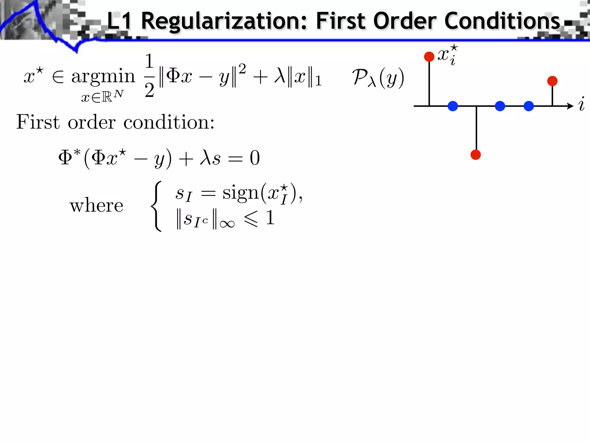
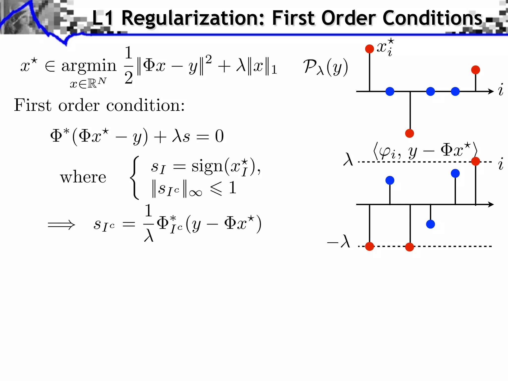
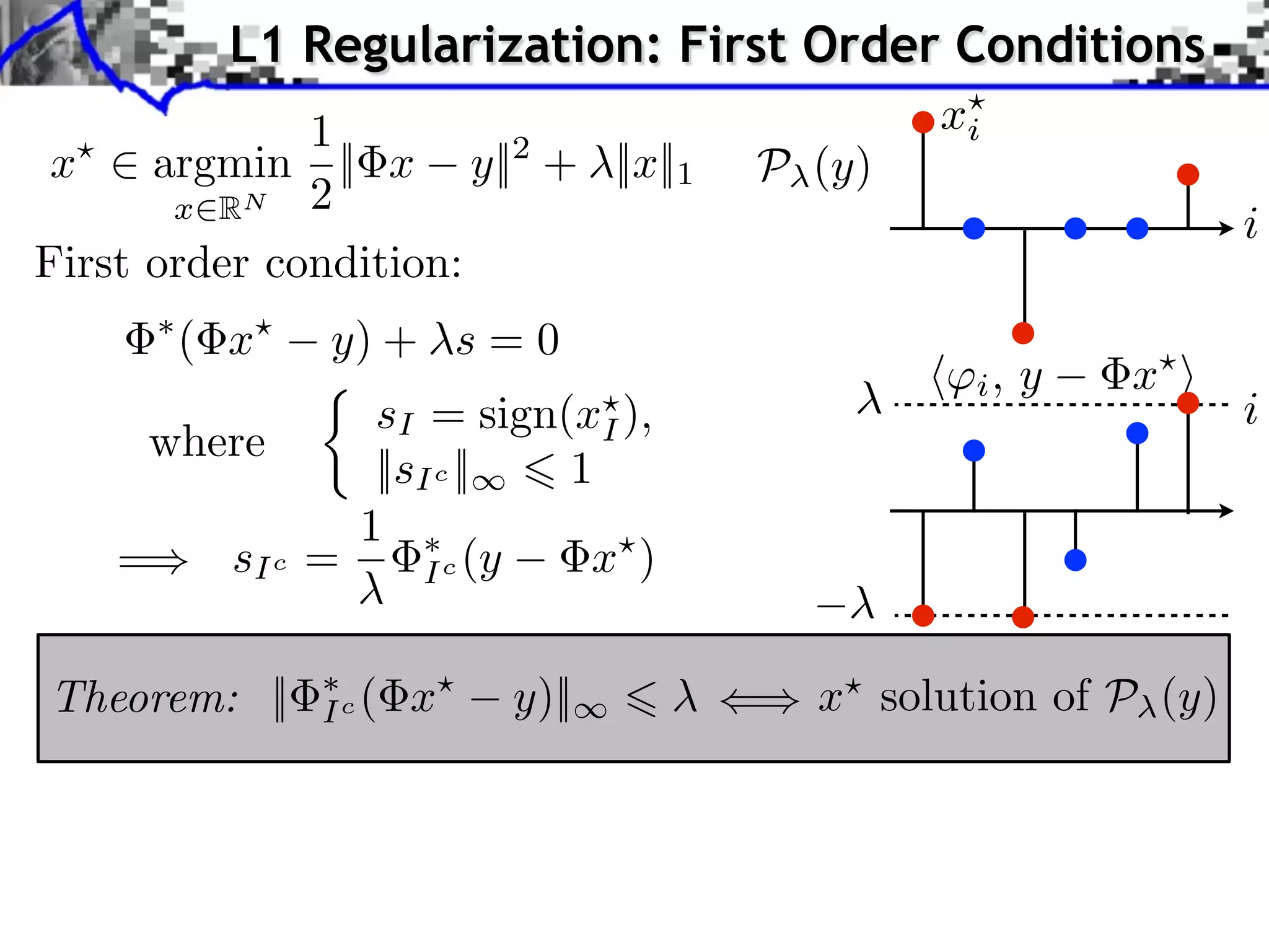
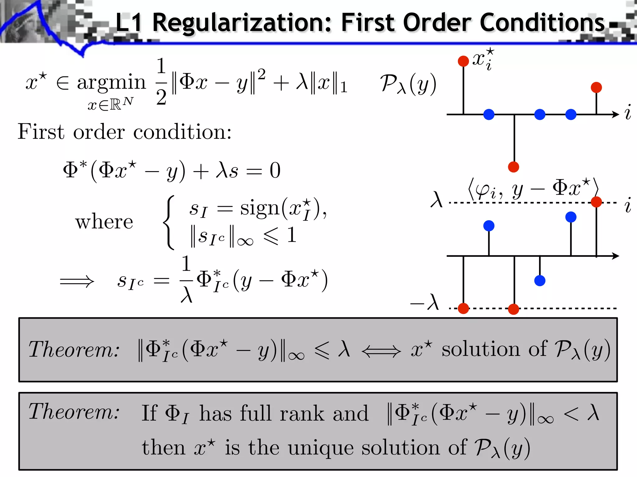
![L1 Regularization: First Order Conditions
1
x ⇥ argmin G(x) = ||y x||2 + ||x||1
x RQ 2
⇥G(x) = ( x y) + ⇥|| · ||1 (x)
sign(xi ) if xi ⇥= 0,
|| · ||1 (x)i =
[ 1, 1] if xi = 0.](https://image.slidesharecdn.com/2012-07-10-centrale-121213050709-phpapp02/75/Sparsity-and-Compressed-Sensing-56-2048.jpg)
![L1 Regularization: First Order Conditions
1
x ⇥ argmin G(x) = ||y x||2 + ||x||1
x RQ 2
⇥G(x) = ( x y) + ⇥|| · ||1 (x)
sign(xi ) if xi ⇥= 0,
|| · ||1 (x)i =
[ 1, 1] if xi = 0.
xi
Support of the solution:
i
I = {i ⇥ {0, . . . , N 1} xi ⇤= 0}](https://image.slidesharecdn.com/2012-07-10-centrale-121213050709-phpapp02/75/Sparsity-and-Compressed-Sensing-57-2048.jpg)
![L1 Regularization: First Order Conditions
1
x ⇥ argmin G(x) = ||y x||2 + ||x||1
x RQ 2
⇥G(x) = ( x y) + ⇥|| · ||1 (x)
sign(xi ) if xi ⇥= 0,
|| · ||1 (x)i =
[ 1, 1] if xi = 0.
xi
Support of the solution:
i
I = {i ⇥ {0, . . . , N 1} xi ⇤= 0}
Restrictions:
xI = (xi )i I R|I| I = ( i )i I RP |I|](https://image.slidesharecdn.com/2012-07-10-centrale-121213050709-phpapp02/75/Sparsity-and-Compressed-Sensing-58-2048.jpg)


![Robustness to Small Noise
Identifiability crition: [Fuchs]
For s ⇥ { 1, 0, +1}N , let I = supp(s)
F(s) = || I sI || where I = Ic
+,
I](https://image.slidesharecdn.com/2012-07-10-centrale-121213050709-phpapp02/75/Sparsity-and-Compressed-Sensing-70-2048.jpg)
![Robustness to Small Noise
Identifiability crition: [Fuchs]
For s ⇥ { 1, 0, +1}N , let I = supp(s)
F(s) = || I sI || where I = Ic
+,
I
Theorem: [Fuchs 2004] If F (sign(x0 )) < 1, T = min |x0,i |
i I
If ||w||/T is small enough and ||w||, then
x0,I + +
I w ( I I)
1
sign(x0,I )
is the unique solution of P (y).](https://image.slidesharecdn.com/2012-07-10-centrale-121213050709-phpapp02/75/Sparsity-and-Compressed-Sensing-71-2048.jpg)
![Robustness to Small Noise
Identifiability crition: [Fuchs]
For s ⇥ { 1, 0, +1}N , let I = supp(s)
F(s) = || I sI || where I = Ic
+,
I
Theorem: [Fuchs 2004] If F (sign(x0 )) < 1, T = min |x0,i |
i I
If ||w||/T is small enough and ||w||, then
x0,I + +
I w ( I I)
1
sign(x0,I )
is the unique solution of P (y).
When w = 0, F (sign(x0 ) < 1 = x = x0 .](https://image.slidesharecdn.com/2012-07-10-centrale-121213050709-phpapp02/75/Sparsity-and-Compressed-Sensing-72-2048.jpg)
![Robustness to Small Noise
Identifiability crition: [Fuchs]
For s ⇥ { 1, 0, +1}N , let I = supp(s)
F(s) = || I sI || where I = Ic
+,
I
Theorem: [Fuchs 2004] If F (sign(x0 )) < 1, T = min |x0,i |
i I
If ||w||/T is small enough and ||w||, then
x0,I + +
I w ( I I)
1
sign(x0,I )
is the unique solution of P (y).
When w = 0, F (sign(x0 ) < 1 = x = x0 .
Theorem: [Grassmair et al. 2010] If F (sign(x0 )) < 1
if ||w||, ||x x0 || = O(||w||)](https://image.slidesharecdn.com/2012-07-10-centrale-121213050709-phpapp02/75/Sparsity-and-Compressed-Sensing-73-2048.jpg)
![Robustness to Bounded Noise
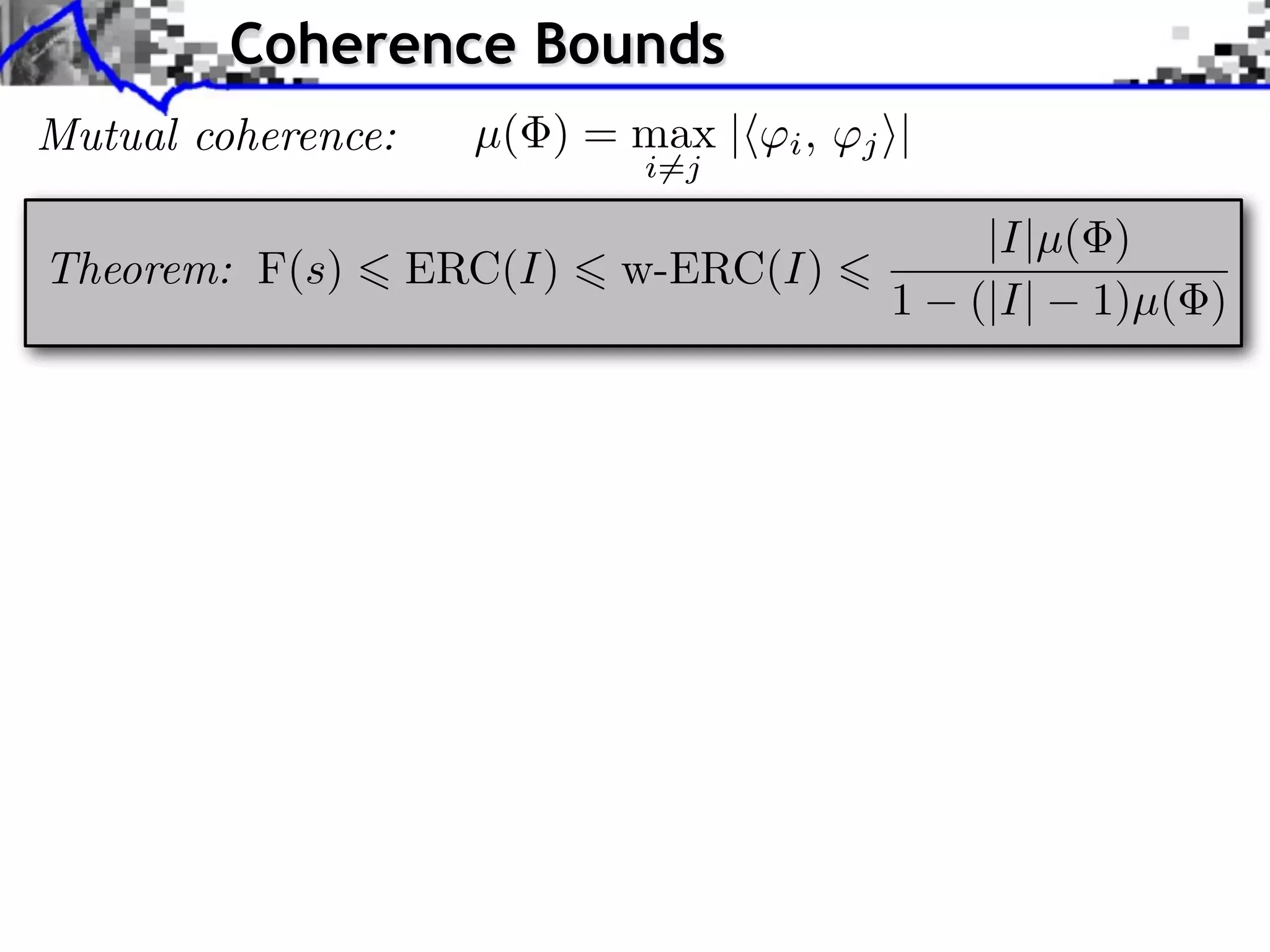
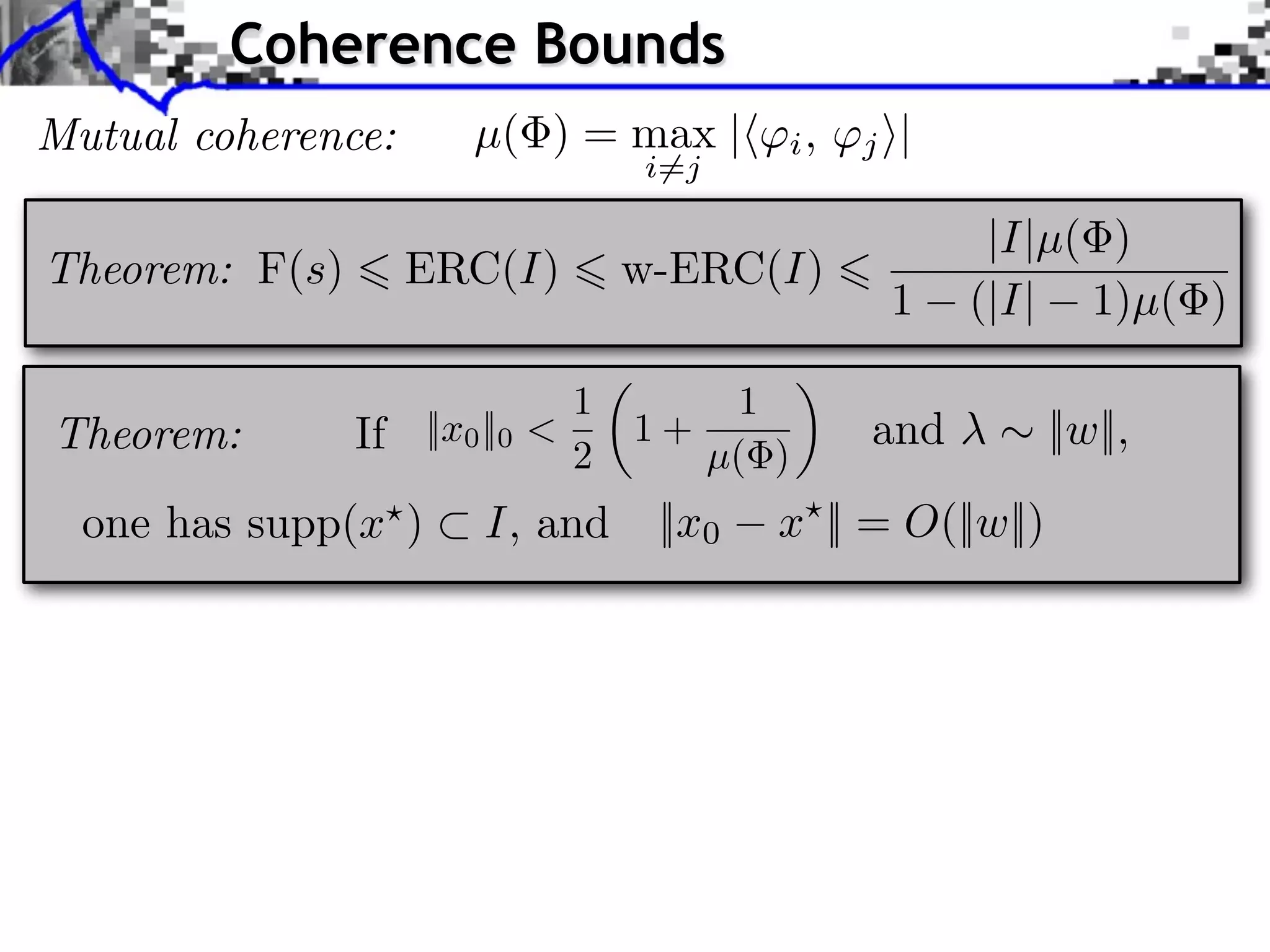
Exact Recovery Criterion (ERC): [Tropp]
For a support I ⇥ {0, . . . , N 1} with I full rank,
ERC(I) = || I || , where I = Ic
+,
I
= || +
I Ic ||1,1 = max ||
c
+
I j ||1
j I
(use ||(aj )j ||1,1 = maxj ||aj ||1 )
Relation with F criterion: ERC(I) = max F(s)
s,supp(s) I](https://image.slidesharecdn.com/2012-07-10-centrale-121213050709-phpapp02/75/Sparsity-and-Compressed-Sensing-77-2048.jpg)
![Robustness to Bounded Noise
Exact Recovery Criterion (ERC): [Tropp]
For a support I ⇥ {0, . . . , N 1} with I full rank,
ERC(I) = || I || , where I = Ic
+,
I
= || +
I Ic ||1,1 = max ||
c
+
I j ||1
j I
(use ||(aj )j ||1,1 = maxj ||aj ||1 )
Relation with F criterion: ERC(I) = max F(s)
s,supp(s) I
Theorem: If ERC(supp(x0 )) < 1 and ||w||, then
x is unique, satisfies supp(x ) supp(x0 ), and
||x0 x || = O(||w||)](https://image.slidesharecdn.com/2012-07-10-centrale-121213050709-phpapp02/75/Sparsity-and-Compressed-Sensing-78-2048.jpg)
![Spikes and Sinusoids Separation
Incoherent pair of orthobases: Diracs/Fourier
2i
1 = {k ⇤⇥ [k m]}m 2 = k N 1/2
e N mk
m
=[ 1, 2] RN 2N](https://image.slidesharecdn.com/2012-07-10-centrale-121213050709-phpapp02/75/Sparsity-and-Compressed-Sensing-84-2048.jpg)
![Spikes and Sinusoids Separation
Incoherent pair of orthobases: Diracs/Fourier
2i
1 = {k ⇤⇥ [k m]}m 2 = k N 1/2
e N mk
m
=[ 1, 2] RN 2N
1
min ||y x||2 + ||x||1
x R2N 2
1
min ||y 1 x1 2 x2 ||2 + ||x1 ||1 + ||x2 ||1
x1 ,x2 RN 2
= +](https://image.slidesharecdn.com/2012-07-10-centrale-121213050709-phpapp02/75/Sparsity-and-Compressed-Sensing-85-2048.jpg)
![Spikes and Sinusoids Separation
Incoherent pair of orthobases: Diracs/Fourier
2i
1 = {k ⇤⇥ [k m]}m 2 = k N 1/2
e N mk
m
=[ 1, 2] RN 2N
1
min ||y x||2 + ||x||1
x R2N 2
1
min ||y 1 x1 2 x2 ||2 + ||x1 ||1 + ||x2 ||1
x1 ,x2 RN 2
= +
1
µ( ) = = separates up to N /2 Diracs + sines.
N](https://image.slidesharecdn.com/2012-07-10-centrale-121213050709-phpapp02/75/Sparsity-and-Compressed-Sensing-86-2048.jpg)
![Pointwise Sampling and Smoothness
Data aquisition: ˜ ˜
f [i] = f (i/N ) = f , i
0
1
Sensors 2
( i )i
(Diracs)
˜
f L2 f RN
ˆ
˜
Shannon interpolation: if Supp(f ) [ N ,N ]](https://image.slidesharecdn.com/2012-07-10-centrale-121213050709-phpapp02/75/Sparsity-and-Compressed-Sensing-88-2048.jpg)
![Pointwise Sampling and Smoothness
Data aquisition: ˜ ˜
f [i] = f (i/N ) = f , i
0
1
Sensors 2
( i )i
(Diracs)
˜
f L2 f RN
ˆ
˜
Shannon interpolation: if Supp(f ) [ N ,N ]
˜
f (t) = f [i]h(N t i)
i
sin( t)
where h(t) =
t](https://image.slidesharecdn.com/2012-07-10-centrale-121213050709-phpapp02/75/Sparsity-and-Compressed-Sensing-89-2048.jpg)
![Pointwise Sampling and Smoothness
Data aquisition: ˜ ˜
f [i] = f (i/N ) = f , i
0
1
Sensors 2
( i )i
(Diracs)
˜
f L2 f RN
ˆ
˜
Shannon interpolation: if Supp(f ) [ N ,N ]
˜
f (t) = f [i]h(N t i)
i
sin( t)
where h(t) =
t
Natural images are not smooth.
But can be compressed e ciently.](https://image.slidesharecdn.com/2012-07-10-centrale-121213050709-phpapp02/75/Sparsity-and-Compressed-Sensing-90-2048.jpg)
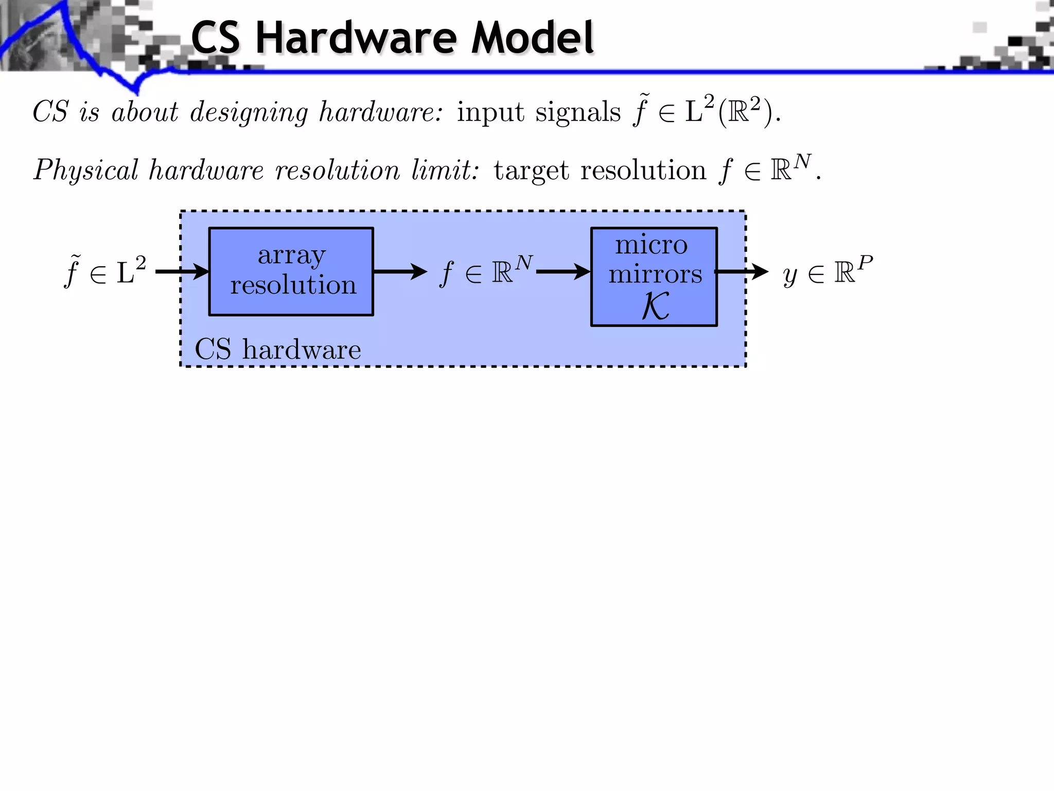
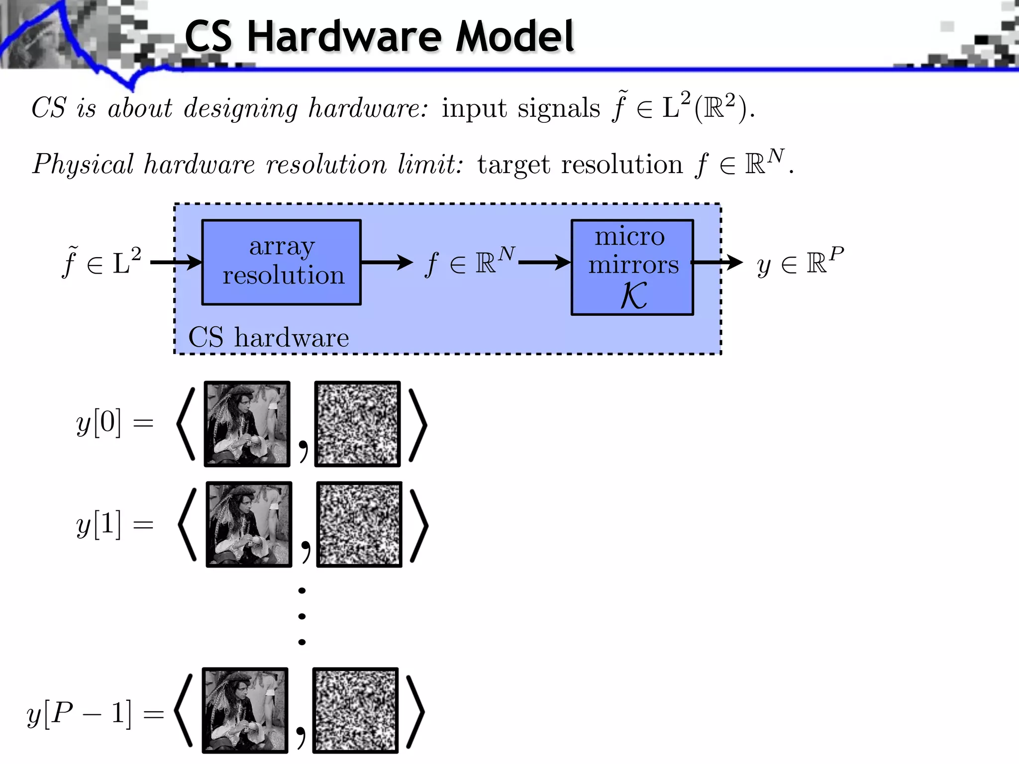
![Single Pixel Camera (Rice)
y[i] = f0 , i⇥](https://image.slidesharecdn.com/2012-07-10-centrale-121213050709-phpapp02/75/Sparsity-and-Compressed-Sensing-91-2048.jpg)
![Single Pixel Camera (Rice)
y[i] = f0 , i⇥
f0 , N = 2562 f , P/N = 0.16 f , P/N = 0.02](https://image.slidesharecdn.com/2012-07-10-centrale-121213050709-phpapp02/75/Sparsity-and-Compressed-Sensing-92-2048.jpg)
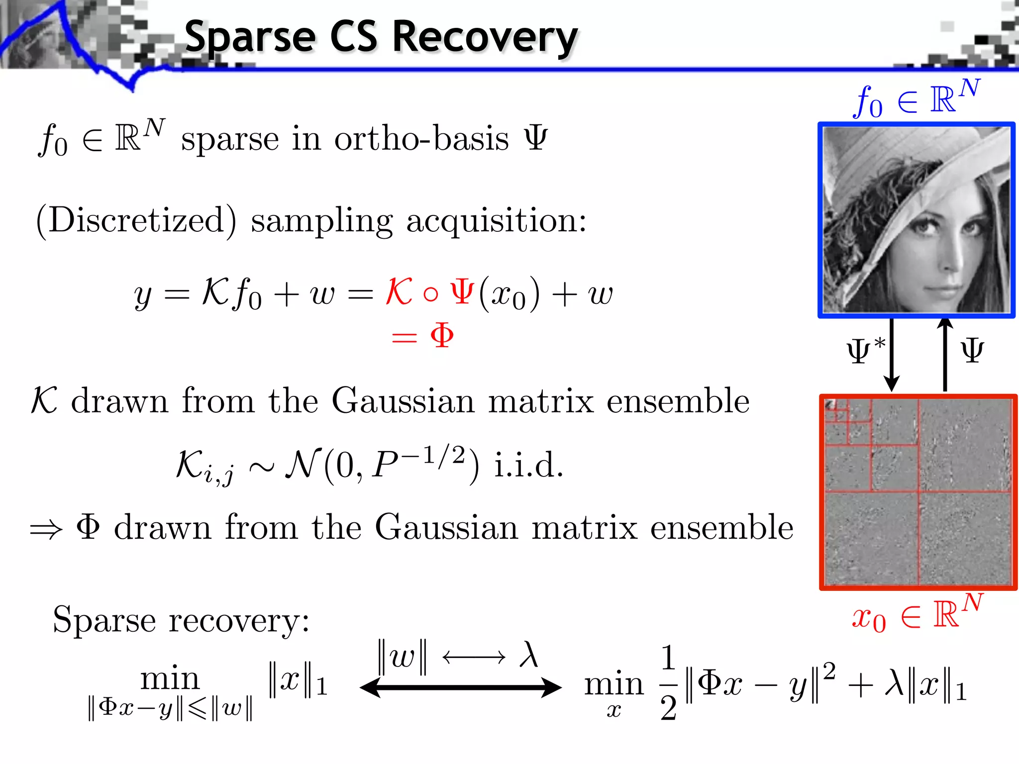
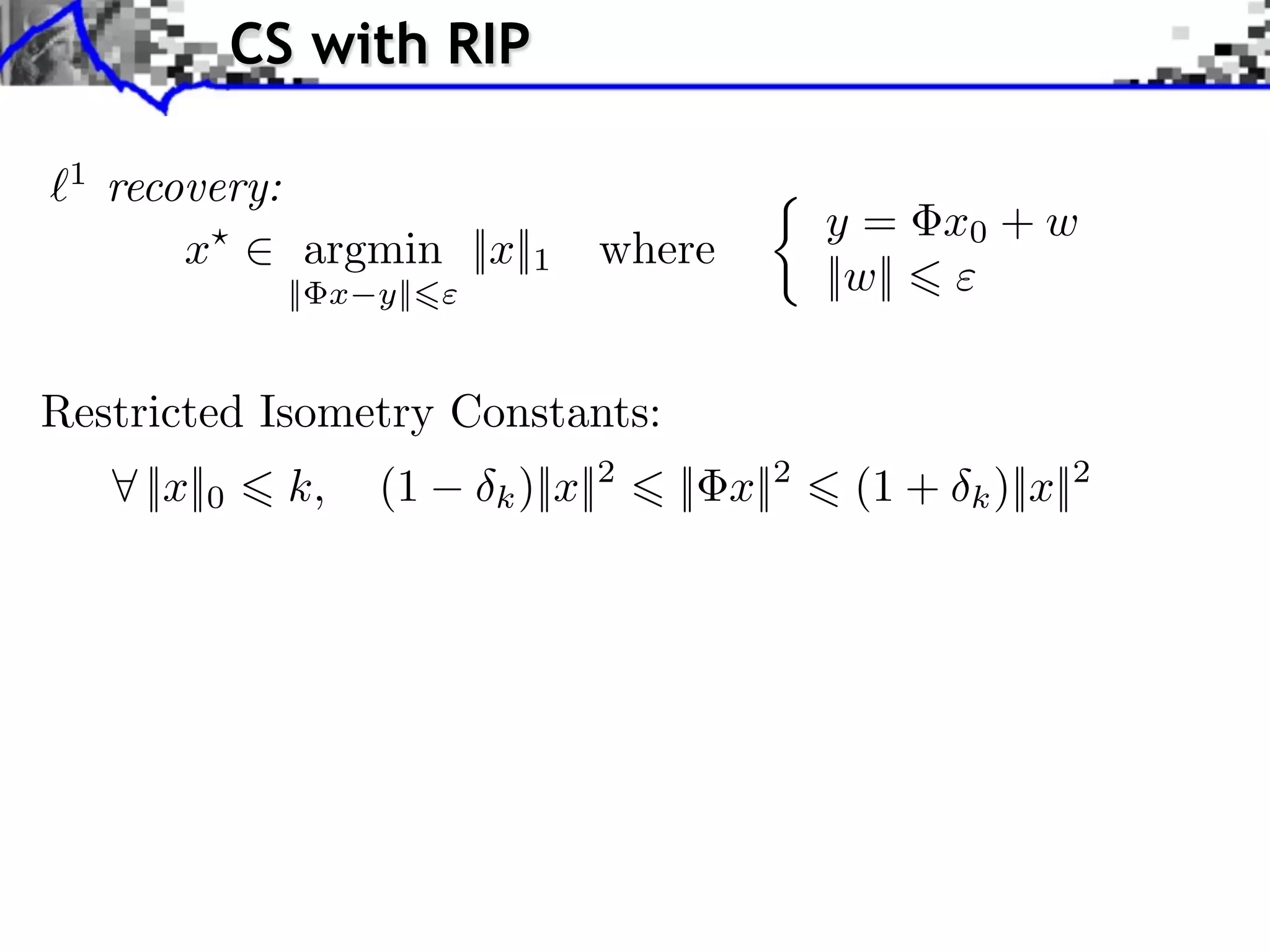
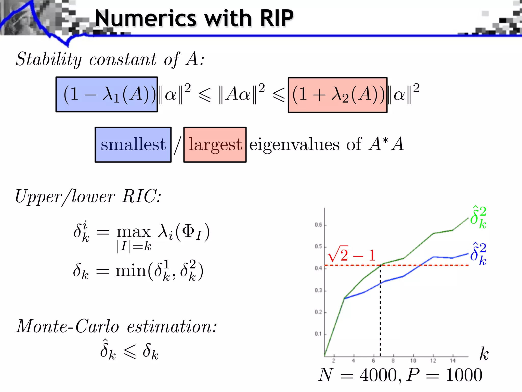
![CS with RIP
1
recovery:
y = x0 + w
x⇥ argmin ||x||1 where
|| x y|| ||w||
Restricted Isometry Constants:
⇥ ||x||0 k, (1 k )||x||2 || x||2 (1 + k )||x||2
Theorem: If 2k 2 1, then [Candes 2009]
C0
||x0 x || ⇥ ||x0 xk ||1 + C1
k
where xk is the best k-term approximation of x0 .](https://image.slidesharecdn.com/2012-07-10-centrale-121213050709-phpapp02/75/Sparsity-and-Compressed-Sensing-103-2048.jpg)
![Singular Values Distributions
Eigenvalues of I I with |I| = k are essentially in [a, b]
a = (1 )2 and b = (1 )2 where = k/P
When k = P + , the eigenvalue distribution tends to
1
f (⇥) = (⇥ b)+ (a ⇥)+ [Marcenko-Pastur]
1.5
2⇤ ⇥ P=200, k=10
P=200, k=10
f ( )
1.5
1
1
0.5
P = 200, k = 10
0.5
0
0 0.5 1 1.5 2 2.5
0
0 0.5 1 P=200, k=30 1.5 2 2.5
1
P=200, k=30
0.8
1
0.6
0.8
0.4
k = 30
0.6
0.2
0.4
0
0.2
0 0.5 1 1.5 2 2.5
0
0 0.5 1 P=200, k=50 1.5 2 2.5
P=200, k=50
0.8
0.8
0.6
0.6
0.4
Large deviation inequality [Ledoux]
0.4
0.2](https://image.slidesharecdn.com/2012-07-10-centrale-121213050709-phpapp02/75/Sparsity-and-Compressed-Sensing-104-2048.jpg)
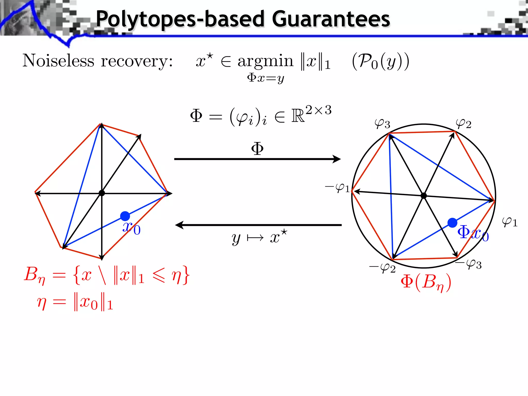
![Polytope Noiseless Recovery
Counting faces of random polytopes: [Donoho]
All x0 such that ||x0 ||0 Call (P/N )P are identifiable.
Most x0 such that ||x0 ||0 Cmost (P/N )P are identifiable.
Call (1/4) 0.065
1
0.9
Cmost (1/4) 0.25 0.8
0.7
0.6
Sharp constants. 0.5
0.4
No noise robustness. 0.3
0.2
0.1
0
50 100 150 200 250 300 350 400
RIP
All Most](https://image.slidesharecdn.com/2012-07-10-centrale-121213050709-phpapp02/75/Sparsity-and-Compressed-Sensing-113-2048.jpg)
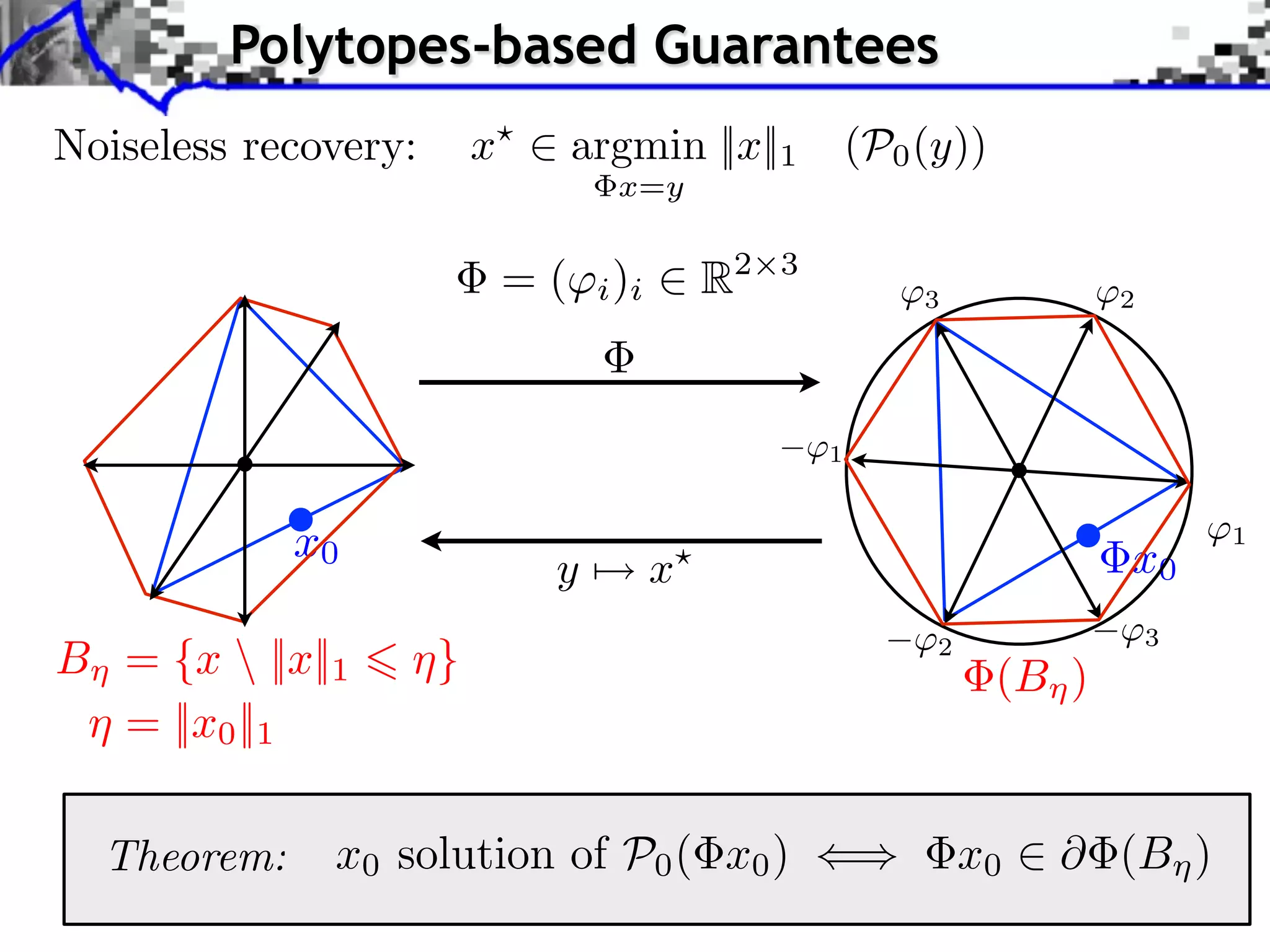
![Polytope Noiseless Recovery
Counting faces of random polytopes: [Donoho]
All x0 such that ||x0 ||0 Call (P/N )P are identifiable.
Most x0 such that ||x0 ||0 Cmost (P/N )P are identifiable.
Call (1/4) 0.065
1
0.9
Cmost (1/4) 0.25 0.8
0.7
0.6
Sharp constants. 0.5
0.4
No noise robustness. 0.3
Computation of
0.2
0.1
“pathological” signals 0
50 100 150 200 250 300 350 400
[Dossal, P, Fadili, 2010]
RIP
All Most](https://image.slidesharecdn.com/2012-07-10-centrale-121213050709-phpapp02/75/Sparsity-and-Compressed-Sensing-114-2048.jpg)
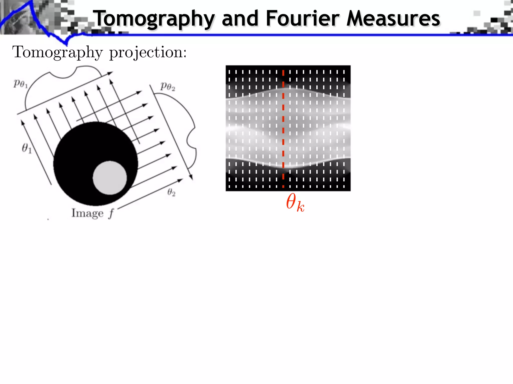
![Tomography and Fourier Measures
ˆ
f = FFT2(f )
k
Fourier slice theorem: ˆ ˆ
p (⇥) = f (⇥ cos( ), ⇥ sin( ))
1D 2D Fourier
R
Partial Fourier measurements: {p k (t)}t
0 k<K
Equivalent to: ˆ
f = {f [ ]}](https://image.slidesharecdn.com/2012-07-10-centrale-121213050709-phpapp02/75/Sparsity-and-Compressed-Sensing-117-2048.jpg)
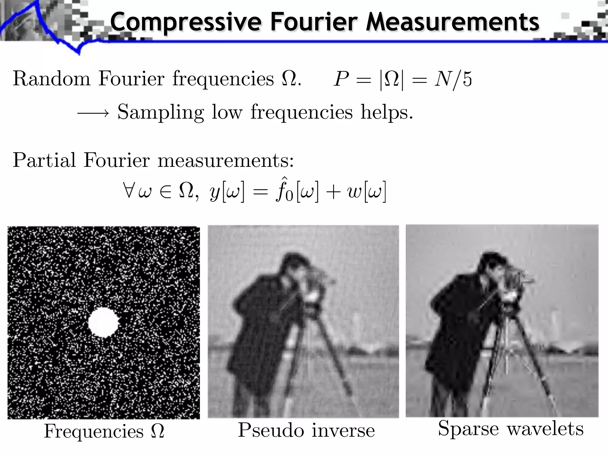
![Regularized Inversion
Noisy measurements: ⇥ ˆ
, y[ ] = f0 [ ] + w[ ].
Noise: w[⇥] N (0, ), white noise.
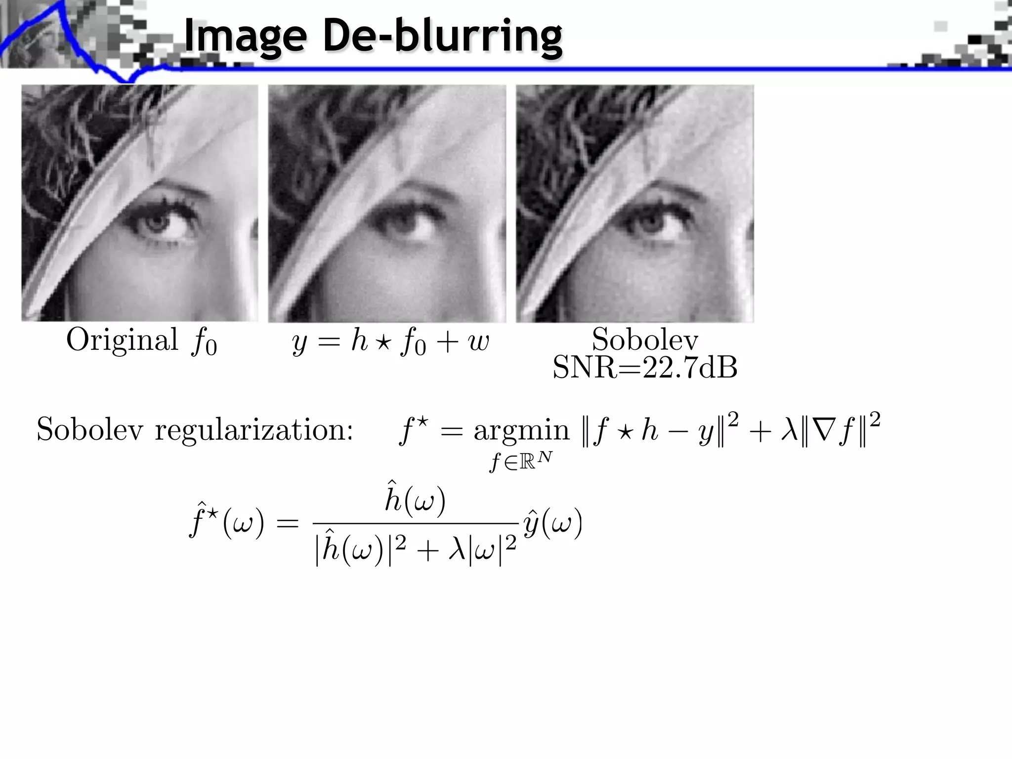
1
regularization:
1 ˆ
f = argmin
⇥
|y[⇤] f [⇤]|2 + |⇥f, ⇥m ⇤|.
f 2 m
+ f
f
Disclaimer: this is not compressed sensing.](https://image.slidesharecdn.com/2012-07-10-centrale-121213050709-phpapp02/75/Sparsity-and-Compressed-Sensing-118-2048.jpg)
![MRI Imaging
From [Lutsig et al.]](https://image.slidesharecdn.com/2012-07-10-centrale-121213050709-phpapp02/75/Sparsity-and-Compressed-Sensing-119-2048.jpg)
![MRI Reconstruction
From [Lutsig et al.]
randomization
Fourier sub-sampling pattern:
High resolution Low resolution Linear Sparsity](https://image.slidesharecdn.com/2012-07-10-centrale-121213050709-phpapp02/75/Sparsity-and-Compressed-Sensing-120-2048.jpg)
![Structured Measurements
Gaussian matrices: intractable for large N .
Random partial orthogonal matrix: { } orthogonal basis.
=( ) where | | = P drawn uniformly at random.
Fast measurements: (e.g. Fourier basis)
, y[ ] = f, ⇥ ˆ
= f[ ]](https://image.slidesharecdn.com/2012-07-10-centrale-121213050709-phpapp02/75/Sparsity-and-Compressed-Sensing-122-2048.jpg)
![Structured Measurements
Gaussian matrices: intractable for large N .
Random partial orthogonal matrix: { } orthogonal basis.
=( ) where | | = P drawn uniformly at random.
Fast measurements: (e.g. Fourier basis)
, ˆ
y[ ] = f, ⇥ = f [ ]
⌅ ⌅
Mutual incoherence: µ = N max |⇥⇥ , m ⇤| [1, N ]
,m](https://image.slidesharecdn.com/2012-07-10-centrale-121213050709-phpapp02/75/Sparsity-and-Compressed-Sensing-123-2048.jpg)
![Structured Measurements
Gaussian matrices: intractable for large N .
Random partial orthogonal matrix: { } orthogonal basis.
=( ) where | | = P drawn uniformly at random.
Fast measurements: (e.g. Fourier basis)
, ˆ
y[ ] = f, ⇥ = f [ ]
⌅ ⌅
Mutual incoherence: µ = N max |⇥⇥ , m ⇤| [1, N ]
,m
Theorem: with high probability on ,
CP
If M 2 log(N )4
, then 2M 2 1
µ
[Rudelson, Vershynin, 2006]
not universal: requires incoherence.](https://image.slidesharecdn.com/2012-07-10-centrale-121213050709-phpapp02/75/Sparsity-and-Compressed-Sensing-124-2048.jpg)
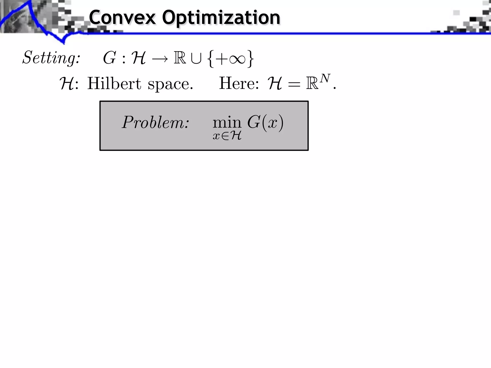
![Convex Optimization
Setting: G : H R ⇤ {+⇥}
H: Hilbert space. Here: H = RN .
Problem: min G(x)
x H
Class of functions: x y
Convex: G(tx + (1 t)y) tG(x) + (1 t)G(y) t [0, 1]](https://image.slidesharecdn.com/2012-07-10-centrale-121213050709-phpapp02/75/Sparsity-and-Compressed-Sensing-127-2048.jpg)
![Convex Optimization
Setting: G : H R ⇤ {+⇥}
H: Hilbert space. Here: H = RN .
Problem: min G(x)
x H
Class of functions: x y
Convex: G(tx + (1 t)y) tG(x) + (1 t)G(y) t [0, 1]
Lower semi-continuous: lim inf G(x) G(x0 )
x x0
Proper: {x ⇥ H G(x) ⇤= + } = ⌅
⇤](https://image.slidesharecdn.com/2012-07-10-centrale-121213050709-phpapp02/75/Sparsity-and-Compressed-Sensing-128-2048.jpg)
![Convex Optimization
Setting: G : H R ⇤ {+⇥}
H: Hilbert space. Here: H = RN .
Problem: min G(x)
x H
Class of functions: x y
Convex: G(tx + (1 t)y) tG(x) + (1 t)G(y) t [0, 1]
Lower semi-continuous: lim inf G(x) G(x0 )
x x0
Proper: {x ⇥ H G(x) ⇤= + } = ⌅
⇤
0 if x ⇥ C,
Indicator: C (x) =
+ otherwise.
(C closed and convex)](https://image.slidesharecdn.com/2012-07-10-centrale-121213050709-phpapp02/75/Sparsity-and-Compressed-Sensing-129-2048.jpg)
![Gradient and Proximal Descents
Gradient descent: x( +1) = x( ) G(x( ) ) [explicit]
G is C 1 and G is L-Lipschitz
Theorem: If 0 < < 2/L, x( )
x a solution.](https://image.slidesharecdn.com/2012-07-10-centrale-121213050709-phpapp02/75/Sparsity-and-Compressed-Sensing-137-2048.jpg)
![Gradient and Proximal Descents
Gradient descent: x( +1) = x( ) G(x( ) ) [explicit]
G is C 1 and G is L-Lipschitz
Theorem: If 0 < < 2/L, x( )
x a solution.
Sub-gradient descent: x( +1)
= x( )
v( ) , v( )
G(x( ) )
Theorem: If 1/⇥, x( )
x a solution.
Problem: slow.](https://image.slidesharecdn.com/2012-07-10-centrale-121213050709-phpapp02/75/Sparsity-and-Compressed-Sensing-138-2048.jpg)
![Gradient and Proximal Descents
Gradient descent: x( +1) = x( ) G(x( ) ) [explicit]
G is C 1 and G is L-Lipschitz
Theorem: If 0 < < 2/L, x( )
x a solution.
Sub-gradient descent: x( +1)
= x( )
v( ) , v( )
G(x( ) )
Theorem: If 1/⇥, x( )
x a solution.
Problem: slow.
Proximal-point algorithm: x(⇥+1) = Prox G (x(⇥) ) [implicit]
Theorem: If c > 0, x( )
x a solution.
Prox G hard to compute.](https://image.slidesharecdn.com/2012-07-10-centrale-121213050709-phpapp02/75/Sparsity-and-Compressed-Sensing-139-2048.jpg)
![RAINED DICTIONARY. THE BOTTOM-RIGHT ARE THE IMPROVEMENTS OBTAINED WITH THE ADAPTIVE APPROACH WITH 20 IT
CALE K-SVD ALGORITHM [2] ON EACH CHANNEL SEPARATELY WITH 8
EPRESENTATION FOR COLOR IMAGE RESTORATION
DENOISING ALGORITHM WITH 256 ATOMS OF SIZE 7 7 3 FOR
ESULTS ARE THOSE GIVEN BY MCAULEY AND AL [28] WITH THEIR “3 Some Hot Topics
color artifacts while reconstructing a damaged version of the image (a) without the improvement here proposed ( in the new metric).
uced with our proposed technique ( in our proposed new metric). Both images have been denoised with the same global dictionary.
bias effect in the color from the castle and in some part of the water. What is more, the color of the sky is piecewise constant when
h is another artifact our approach corrected. (a) Original. (b) Original algorithm, dB. (c) Proposed algorithm,
Dictionary learning:
dB.
with 256 atoms learned on a generic database of natural images, with two different sizes ofREPRESENTATION FOR COLOR IMAGE RESTORATION
MAIRAL et al.: SPARSE patches. Note the large number of color-less atoms. 57
ave negative values, the vectors are presented scaled and shifted to the [0,255] range per channel: (a) 5 5 3 patches; (b) 8 8 3 patches.
R IMAGE RESTORATION 61
Fig. 7. Data set used for evaluating denoising experiments.
learning
ing Image; (b) resulting dictionary; (b) is the dictionary learned in the image in (a). The dictionary is more colored than the global one.
TABLE I
g. 7. Data set used for evaluating denoising experiments. with 256 atoms learned on a generic database of natural images, with two different sizes of patches. Note the large number of color-less atoms.
Fig. 2. Dictionaries
Since the atoms can have negative values, the vectors are presented scaled and shifted to the [0,255] range per channel: (a) 5 5 3 patches; (b) 8 8 3 patches.
color artifacts while reconstructing a damaged version of the image (a) without the improvement here proposed ( in the new metric).
duced with our proposed technique (
TABLE I our proposed new metric). Both images have been denoised with the same global dictionary.
in
TH 256 ATOMS OF SIZE castle 7 in3 FOR of the water. What is more, the color of the sky is.piecewise CASE IS DIVIDED IN FOUR
a bias effect in the color from the 7 and some part AND 6 6 3 FOR EACH constant when
ch is another artifact our approach corrected. (a)HEIR “3(b) Original algorithm, HE TOP-RIGHT RESULTS ARE THOSE OBTAINED BY
Y MCAULEY AND AL [28] WITH T Original. 3 MODEL.” T dB. (c) Proposed algorithm,
3 MODEL.” THE TOP-RIGHT RESULTS ARE THOSE O
dB.
8 ATOMS. THE BOTTOM-LEFT ARE OUR RESULTS
2] ON EACH CHANNEL SEPARATELY WITH 8 8 ATOMS. THE BOTTOM-LEFT ARE OUR RESULTS OBTAINED
AND 6
OTTOM-RIGHT ARE THE IMPROVEMENTS OBTAINED WITH THE ADAPTIVE APPROACH WITH 20 ITERATIONS.
H GROUP. AS CAN BE SEEN, OUR PROPOSED TECHNIQUE CONSISTENTLY PRODUCES THE BEST RESULTS
6 3 FOR
Fig. 3. Examples of color artifacts while reconstructing a damaged version of the image (a) without the improvement here proposed ( in the new metric).
Color artifacts are reduced with our proposed technique ( in our proposed new metric). Both images have been denoised with the same global dictionary.
In (b), one observes a bias effect in the color from the castle and in some part of the water. What is more, the color of the sky is piecewise constant when
(false contours), which is another artifact our approach corrected. (a) Original. (b) Original algorithm, dB. (c) Proposed algorithm,
dB.
. EACH CASE IS DIVID](https://image.slidesharecdn.com/2012-07-10-centrale-121213050709-phpapp02/75/Sparsity-and-Compressed-Sensing-163-2048.jpg)
![RAINED DICTIONARY. THE BOTTOM-RIGHT ARE THE IMPROVEMENTS OBTAINED WITH THE ADAPTIVE APPROACH WITH 20 IT
CALE K-SVD ALGORITHM [2] ON EACH CHANNEL SEPARATELY WITH 8
EPRESENTATION FOR COLOR IMAGE RESTORATION
DENOISING ALGORITHM WITH 256 ATOMS OF SIZE 7 7 3 FOR
ESULTS ARE THOSE GIVEN BY MCAULEY AND AL [28] WITH THEIR “3 Some Hot Topics
color artifacts while reconstructing a damaged version of the image (a) without the improvement here proposed ( in the new metric).
uced with our proposed technique ( in our proposed new metric). Both images have been denoised with the same global dictionary.
bias effect in the color from the castle and in some part of the water. What is more, the color of the sky is piecewise constant when
Image f =
h is another artifact our approach corrected. (a) Original. (b) Original algorithm, dB. (c) Proposed algorithm,
dB.
Dictionary learning:
with 256 atoms learned on a generic database of natural images, with two different sizes ofREPRESENTATION FOR COLOR IMAGE RESTORATION
ave negative values, the vectors are presented scaled and shifted to the [0,255] range per channel: (a) 5
MAIRAL et al.: SPARSE patches. Note the large number of color-less
5 3 patches; (b) 8 8
atoms.
3 patches.
57
x
R IMAGE RESTORATION 61
Fig. 7. Data set used for evaluating denoising experiments.
learning
ing Image; (b) resulting dictionary; (b) is the dictionary learned in the image in (a). The dictionary is more colored than the global one.
TABLE I
Analysis vs. synthesis:
g. 7. Data set used for evaluating denoising experiments. with 256 atoms learned on a generic database of natural images, with two different sizes of patches. Note the large number of color-less atoms.
Fig. 2. Dictionaries
Since the atoms can have negative values, the vectors are presented scaled and shifted to the [0,255] range per channel: (a) 5 5 3 patches; (b) 8 8 3 patches.
Js (f ) = min ||x||1
color artifacts while reconstructing a damaged version of the image (a) without the improvement here proposed (
TABLE I in the new metric).
duced with our proposed technique (
a bias effect in the color from the 7
in our proposed new metric). Both images have been denoised with the same global dictionary.
TH 256 ATOMS OF SIZE castle 7 in3 FOR of the water. What is more, the color of the sky is.piecewise CASE IS DIVIDED IN FOUR
and some part AND 6 6 3 FOR EACH constant when
f= x
ch is another artifact our approach corrected. (a)HEIR “3(b) Original algorithm, HE TOP-RIGHT RESULTS ARE THOSE OBTAINED BY
Y MCAULEY AND AL [28] WITH T Original. 3 MODEL.” T dB. (c) Proposed algorithm,
3 MODEL.” THE TOP-RIGHT RESULTS ARE THOSE O
dB.
8 ATOMS. THE BOTTOM-LEFT ARE OUR RESULTS
2] ON EACH CHANNEL SEPARATELY WITH 8 8 ATOMS. THE BOTTOM-LEFT ARE OUR RESULTS OBTAINED
AND 6
OTTOM-RIGHT ARE THE IMPROVEMENTS OBTAINED WITH THE ADAPTIVE APPROACH WITH 20 ITERATIONS.
H GROUP. AS CAN BE SEEN, OUR PROPOSED TECHNIQUE CONSISTENTLY PRODUCES THE BEST RESULTS
Coe cients x
6 3 FOR
Fig. 3. Examples of color artifacts while reconstructing a damaged version of the image (a) without the improvement here proposed ( in the new metric).
Color artifacts are reduced with our proposed technique ( in our proposed new metric). Both images have been denoised with the same global dictionary.
In (b), one observes a bias effect in the color from the castle and in some part of the water. What is more, the color of the sky is piecewise constant when
(false contours), which is another artifact our approach corrected. (a) Original. (b) Original algorithm, dB. (c) Proposed algorithm,
dB.
. EACH CASE IS DIVID](https://image.slidesharecdn.com/2012-07-10-centrale-121213050709-phpapp02/75/Sparsity-and-Compressed-Sensing-164-2048.jpg)
![RAINED DICTIONARY. THE BOTTOM-RIGHT ARE THE IMPROVEMENTS OBTAINED WITH THE ADAPTIVE APPROACH WITH 20 IT
CALE K-SVD ALGORITHM [2] ON EACH CHANNEL SEPARATELY WITH 8
EPRESENTATION FOR COLOR IMAGE RESTORATION
DENOISING ALGORITHM WITH 256 ATOMS OF SIZE 7 7 3 FOR
ESULTS ARE THOSE GIVEN BY MCAULEY AND AL [28] WITH THEIR “3 Some Hot Topics
color artifacts while reconstructing a damaged version of the image (a) without the improvement here proposed ( in the new metric).
uced with our proposed technique ( in our proposed new metric). Both images have been denoised with the same global dictionary.
bias effect in the color from the castle and in some part of the water. What is more, the color of the sky is piecewise constant when
Image f =
h is another artifact our approach corrected. (a) Original. (b) Original algorithm, dB. (c) Proposed algorithm,
dB.
Dictionary learning:
with 256 atoms learned on a generic database of natural images, with two different sizes ofREPRESENTATION FOR COLOR IMAGE RESTORATION
ave negative values, the vectors are presented scaled and shifted to the [0,255] range per channel: (a) 5
MAIRAL et al.: SPARSE patches. Note the large number of color-less
5 3 patches; (b) 8 8
atoms.
3 patches.
57
x
R IMAGE RESTORATION 61
Fig. 7. Data set used for evaluating denoising experiments.
learning
D
ing Image; (b) resulting dictionary; (b) is the dictionary learned in the image in (a). The dictionary is more colored than the global one.
TABLE I
Analysis vs. synthesis:
g. 7. Data set used for evaluating denoising experiments. with 256 atoms learned on a generic database of natural images, with two different sizes of patches. Note the large number of color-less atoms.
Fig. 2. Dictionaries
Since the atoms can have negative values, the vectors are presented scaled and shifted to the [0,255] range per channel: (a) 5 5 3 patches; (b) 8 8 3 patches.
Js (f ) = min ||x||1
color artifacts while reconstructing a damaged version of the image (a) without the improvement here proposed (
TABLE I in the new metric).
duced with our proposed technique (
a bias effect in the color from the 7
in our proposed new metric). Both images have been denoised with the same global dictionary.
TH 256 ATOMS OF SIZE castle 7 in3 FOR of the water. What is more, the color of the sky is.piecewise CASE IS DIVIDED IN FOUR
and some part AND 6 6 3 FOR EACH constant when
f= x
J (f ) = ||D f ||
ch is another artifact our approach corrected. (a)HEIR “3(b) Original algorithm, HE TOP-RIGHT RESULTS ARE THOSE OBTAINED BY
Y MCAULEY AND AL [28] WITH T Original. 3 MODEL.” T dB. (c) Proposed algorithm,
3 MODEL.” THE TOP-RIGHT RESULTS ARE THOSE O
dB.
8 ATOMS. THE BOTTOM-LEFT ARE OUR RESULTS
a 1
2] ON EACH CHANNEL SEPARATELY WITH 8 8 ATOMS. THE BOTTOM-LEFT ARE OUR RESULTS OBTAINED
AND 6
OTTOM-RIGHT ARE THE IMPROVEMENTS OBTAINED WITH THE ADAPTIVE APPROACH WITH 20 ITERATIONS.
H GROUP. AS CAN BE SEEN, OUR PROPOSED TECHNIQUE CONSISTENTLY PRODUCES THE BEST RESULTS
Coe cients x c=D f
6 3 FOR
Fig. 3. Examples of color artifacts while reconstructing a damaged version of the image (a) without the improvement here proposed ( in the new metric).
Color artifacts are reduced with our proposed technique ( in our proposed new metric). Both images have been denoised with the same global dictionary.
In (b), one observes a bias effect in the color from the castle and in some part of the water. What is more, the color of the sky is piecewise constant when
(false contours), which is another artifact our approach corrected. (a) Original. (b) Original algorithm, dB. (c) Proposed algorithm,
dB.
. EACH CASE IS DIVID](https://image.slidesharecdn.com/2012-07-10-centrale-121213050709-phpapp02/75/Sparsity-and-Compressed-Sensing-165-2048.jpg)
![RAINED DICTIONARY. THE BOTTOM-RIGHT ARE THE IMPROVEMENTS OBTAINED WITH THE ADAPTIVE APPROACH WITH 20 IT
CALE K-SVD ALGORITHM [2] ON EACH CHANNEL SEPARATELY WITH 8
EPRESENTATION FOR COLOR IMAGE RESTORATION
DENOISING ALGORITHM WITH 256 ATOMS OF SIZE 7 7 3 FOR
ESULTS ARE THOSE GIVEN BY MCAULEY AND AL [28] WITH THEIR “3 Some Hot Topics
color artifacts while reconstructing a damaged version of the image (a) without the improvement here proposed ( in the new metric).
uced with our proposed technique ( in our proposed new metric). Both images have been denoised with the same global dictionary.
bias effect in the color from the castle and in some part of the water. What is more, the color of the sky is piecewise constant when
Image f =
h is another artifact our approach corrected. (a) Original. (b) Original algorithm, dB. (c) Proposed algorithm,
dB.
Dictionary learning:
with 256 atoms learned on a generic database of natural images, with two different sizes ofREPRESENTATION FOR COLOR IMAGE RESTORATION
ave negative values, the vectors are presented scaled and shifted to the [0,255] range per channel: (a) 5
MAIRAL et al.: SPARSE patches. Note the large number of color-less
5 3 patches; (b) 8 8
atoms.
3 patches.
57
x
R IMAGE RESTORATION 61
Fig. 7. Data set used for evaluating denoising experiments.
learning
D
ing Image; (b) resulting dictionary; (b) is the dictionary learned in the image in (a). The dictionary is more colored than the global one.
TABLE I
Analysis vs. synthesis:
g. 7. Data set used for evaluating denoising experiments. with 256 atoms learned on a generic database of natural images, with two different sizes of patches. Note the large number of color-less atoms.
Fig. 2. Dictionaries
Since the atoms can have negative values, the vectors are presented scaled and shifted to the [0,255] range per channel: (a) 5 5 3 patches; (b) 8 8 3 patches.
Js (f ) = min ||x||1
color artifacts while reconstructing a damaged version of the image (a) without the improvement here proposed (
TABLE I in the new metric).
duced with our proposed technique (
a bias effect in the color from the 7
in our proposed new metric). Both images have been denoised with the same global dictionary.
TH 256 ATOMS OF SIZE castle 7 in3 FOR of the water. What is more, the color of the sky is.piecewise CASE IS DIVIDED IN FOUR
and some part AND 6 6 3 FOR EACH constant when
f= x
J (f ) = ||D f ||
ch is another artifact our approach corrected. (a)HEIR “3(b) Original algorithm, HE TOP-RIGHT RESULTS ARE THOSE OBTAINED BY
Y MCAULEY AND AL [28] WITH T Original. 3 MODEL.” T dB. (c) Proposed algorithm,
3 MODEL.” THE TOP-RIGHT RESULTS ARE THOSE O
dB.
8 ATOMS. THE BOTTOM-LEFT ARE OUR RESULTS
a 1
2] ON EACH CHANNEL SEPARATELY WITH 8 8 ATOMS. THE BOTTOM-LEFT ARE OUR RESULTS OBTAINED
AND 6
OTTOM-RIGHT ARE THE IMPROVEMENTS OBTAINED WITH THE ADAPTIVE APPROACH WITH 20 ITERATIONS.
Other sparse priors:
H GROUP. AS CAN BE SEEN, OUR PROPOSED TECHNIQUE CONSISTENTLY PRODUCES THE BEST RESULTS
Coe cients x c=D f
6 3 FOR
Fig. 3. Examples of color artifacts while reconstructing a damaged version of the image (a) without the improvement here proposed ( in the new metric).
Color artifacts are reduced with our proposed technique ( in our proposed new metric). Both images have been denoised with the same global dictionary.
In (b), one observes a bias effect in the color from the castle and in some part of the water. What is more, the color of the sky is piecewise constant when
(false contours), which is another artifact our approach corrected. (a) Original. (b) Original algorithm, dB. (c) Proposed algorithm,
dB.
. EACH CASE IS DIVID
|x1 | + |x2 | max(|x1 |, |x2 |)](https://image.slidesharecdn.com/2012-07-10-centrale-121213050709-phpapp02/75/Sparsity-and-Compressed-Sensing-166-2048.jpg)
![RAINED DICTIONARY. THE BOTTOM-RIGHT ARE THE IMPROVEMENTS OBTAINED WITH THE ADAPTIVE APPROACH WITH 20 IT
CALE K-SVD ALGORITHM [2] ON EACH CHANNEL SEPARATELY WITH 8
EPRESENTATION FOR COLOR IMAGE RESTORATION
DENOISING ALGORITHM WITH 256 ATOMS OF SIZE 7 7 3 FOR
ESULTS ARE THOSE GIVEN BY MCAULEY AND AL [28] WITH THEIR “3 Some Hot Topics
color artifacts while reconstructing a damaged version of the image (a) without the improvement here proposed ( in the new metric).
uced with our proposed technique ( in our proposed new metric). Both images have been denoised with the same global dictionary.
bias effect in the color from the castle and in some part of the water. What is more, the color of the sky is piecewise constant when
Image f =
h is another artifact our approach corrected. (a) Original. (b) Original algorithm, dB. (c) Proposed algorithm,
dB.
Dictionary learning:
with 256 atoms learned on a generic database of natural images, with two different sizes ofREPRESENTATION FOR COLOR IMAGE RESTORATION
ave negative values, the vectors are presented scaled and shifted to the [0,255] range per channel: (a) 5
MAIRAL et al.: SPARSE patches. Note the large number of color-less
5 3 patches; (b) 8 8
atoms.
3 patches.
57
x
R IMAGE RESTORATION 61
Fig. 7. Data set used for evaluating denoising experiments.
learning
D
ing Image; (b) resulting dictionary; (b) is the dictionary learned in the image in (a). The dictionary is more colored than the global one.
TABLE I
Analysis vs. synthesis:
g. 7. Data set used for evaluating denoising experiments. with 256 atoms learned on a generic database of natural images, with two different sizes of patches. Note the large number of color-less atoms.
Fig. 2. Dictionaries
Since the atoms can have negative values, the vectors are presented scaled and shifted to the [0,255] range per channel: (a) 5 5 3 patches; (b) 8 8 3 patches.
Js (f ) = min ||x||1
color artifacts while reconstructing a damaged version of the image (a) without the improvement here proposed (
TABLE I in the new metric).
duced with our proposed technique (
a bias effect in the color from the 7
in our proposed new metric). Both images have been denoised with the same global dictionary.
TH 256 ATOMS OF SIZE castle 7 in3 FOR of the water. What is more, the color of the sky is.piecewise CASE IS DIVIDED IN FOUR
and some part AND 6 6 3 FOR EACH constant when
f= x
J (f ) = ||D f ||
ch is another artifact our approach corrected. (a)HEIR “3(b) Original algorithm, HE TOP-RIGHT RESULTS ARE THOSE OBTAINED BY
Y MCAULEY AND AL [28] WITH T Original. 3 MODEL.” T dB. (c) Proposed algorithm,
3 MODEL.” THE TOP-RIGHT RESULTS ARE THOSE O
dB.
8 ATOMS. THE BOTTOM-LEFT ARE OUR RESULTS
a 1
2] ON EACH CHANNEL SEPARATELY WITH 8 8 ATOMS. THE BOTTOM-LEFT ARE OUR RESULTS OBTAINED
AND 6
OTTOM-RIGHT ARE THE IMPROVEMENTS OBTAINED WITH THE ADAPTIVE APPROACH WITH 20 ITERATIONS.
Other sparse priors:
H GROUP. AS CAN BE SEEN, OUR PROPOSED TECHNIQUE CONSISTENTLY PRODUCES THE BEST RESULTS
Coe cients x c=D f
6 3 FOR
Fig. 3. Examples of color artifacts while reconstructing a damaged version of the image (a) without the improvement here proposed ( in the new metric).
Color artifacts are reduced with our proposed technique ( in our proposed new metric). Both images have been denoised with the same global dictionary.
In (b), one observes a bias effect in the color from the castle and in some part of the water. What is more, the color of the sky is piecewise constant when
(false contours), which is another artifact our approach corrected. (a) Original. (b) Original algorithm, dB. (c) Proposed algorithm,
dB.
. EACH CASE IS DIVID
2 1
|x1 | + |x2 | max(|x1 |, |x2 |) |x1 | + (x2
2 + x3 ) 2](https://image.slidesharecdn.com/2012-07-10-centrale-121213050709-phpapp02/75/Sparsity-and-Compressed-Sensing-167-2048.jpg)
![RAINED DICTIONARY. THE BOTTOM-RIGHT ARE THE IMPROVEMENTS OBTAINED WITH THE ADAPTIVE APPROACH WITH 20 IT
CALE K-SVD ALGORITHM [2] ON EACH CHANNEL SEPARATELY WITH 8
EPRESENTATION FOR COLOR IMAGE RESTORATION
DENOISING ALGORITHM WITH 256 ATOMS OF SIZE 7 7 3 FOR
ESULTS ARE THOSE GIVEN BY MCAULEY AND AL [28] WITH THEIR “3 Some Hot Topics
color artifacts while reconstructing a damaged version of the image (a) without the improvement here proposed ( in the new metric).
uced with our proposed technique ( in our proposed new metric). Both images have been denoised with the same global dictionary.
bias effect in the color from the castle and in some part of the water. What is more, the color of the sky is piecewise constant when
Image f =
h is another artifact our approach corrected. (a) Original. (b) Original algorithm, dB. (c) Proposed algorithm,
dB.
Dictionary learning:
with 256 atoms learned on a generic database of natural images, with two different sizes ofREPRESENTATION FOR COLOR IMAGE RESTORATION
ave negative values, the vectors are presented scaled and shifted to the [0,255] range per channel: (a) 5
MAIRAL et al.: SPARSE patches. Note the large number of color-less
5 3 patches; (b) 8 8
atoms.
3 patches.
57
x
R IMAGE RESTORATION 61
Fig. 7. Data set used for evaluating denoising experiments.
learning
D
ing Image; (b) resulting dictionary; (b) is the dictionary learned in the image in (a). The dictionary is more colored than the global one.
TABLE I
Analysis vs. synthesis:
g. 7. Data set used for evaluating denoising experiments. with 256 atoms learned on a generic database of natural images, with two different sizes of patches. Note the large number of color-less atoms.
Fig. 2. Dictionaries
Since the atoms can have negative values, the vectors are presented scaled and shifted to the [0,255] range per channel: (a) 5 5 3 patches; (b) 8 8 3 patches.
Js (f ) = min ||x||1
color artifacts while reconstructing a damaged version of the image (a) without the improvement here proposed (
TABLE I in the new metric).
duced with our proposed technique (
a bias effect in the color from the 7
in our proposed new metric). Both images have been denoised with the same global dictionary.
TH 256 ATOMS OF SIZE castle 7 in3 FOR of the water. What is more, the color of the sky is.piecewise CASE IS DIVIDED IN FOUR
and some part AND 6 6 3 FOR EACH constant when
f= x
J (f ) = ||D f ||
ch is another artifact our approach corrected. (a)HEIR “3(b) Original algorithm, HE TOP-RIGHT RESULTS ARE THOSE OBTAINED BY
Y MCAULEY AND AL [28] WITH T Original. 3 MODEL.” T dB. (c) Proposed algorithm,
3 MODEL.” THE TOP-RIGHT RESULTS ARE THOSE O
dB.
8 ATOMS. THE BOTTOM-LEFT ARE OUR RESULTS
a 1
2] ON EACH CHANNEL SEPARATELY WITH 8 8 ATOMS. THE BOTTOM-LEFT ARE OUR RESULTS OBTAINED
AND 6
OTTOM-RIGHT ARE THE IMPROVEMENTS OBTAINED WITH THE ADAPTIVE APPROACH WITH 20 ITERATIONS.
Other sparse priors:
H GROUP. AS CAN BE SEEN, OUR PROPOSED TECHNIQUE CONSISTENTLY PRODUCES THE BEST RESULTS
Coe cients x c=D f
6 3 FOR
Fig. 3. Examples of color artifacts while reconstructing a damaged version of the image (a) without the improvement here proposed ( in the new metric).
Color artifacts are reduced with our proposed technique ( in our proposed new metric). Both images have been denoised with the same global dictionary.
In (b), one observes a bias effect in the color from the castle and in some part of the water. What is more, the color of the sky is piecewise constant when
(false contours), which is another artifact our approach corrected. (a) Original. (b) Original algorithm, dB. (c) Proposed algorithm,
dB.
. EACH CASE IS DIVID
2 1
|x1 | + |x2 | max(|x1 |, |x2 |) |x1 | + (x2
2 + x3 ) 2 Nuclear](https://image.slidesharecdn.com/2012-07-10-centrale-121213050709-phpapp02/75/Sparsity-and-Compressed-Sensing-168-2048.jpg)

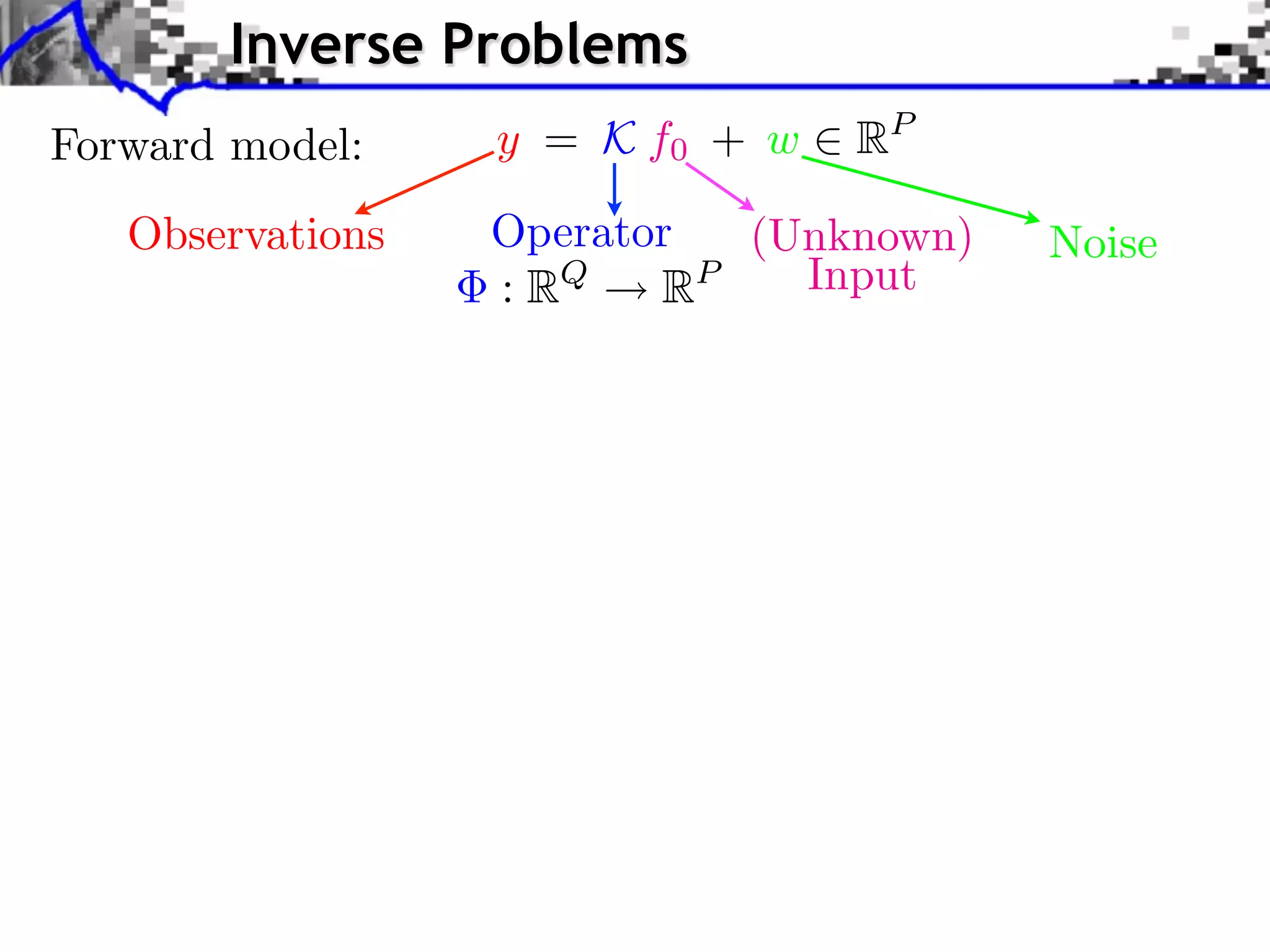
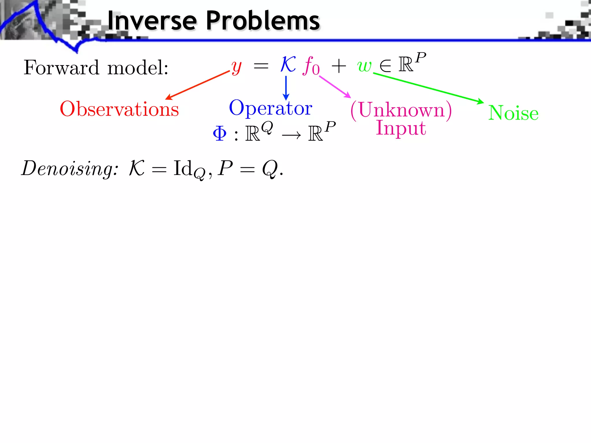
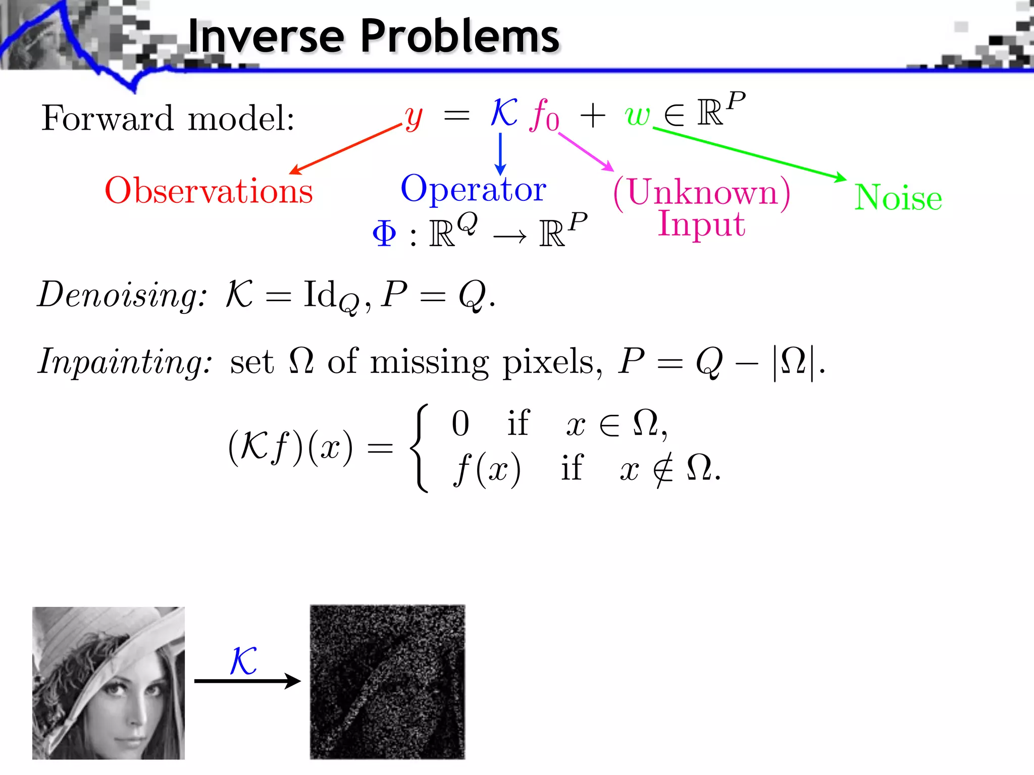
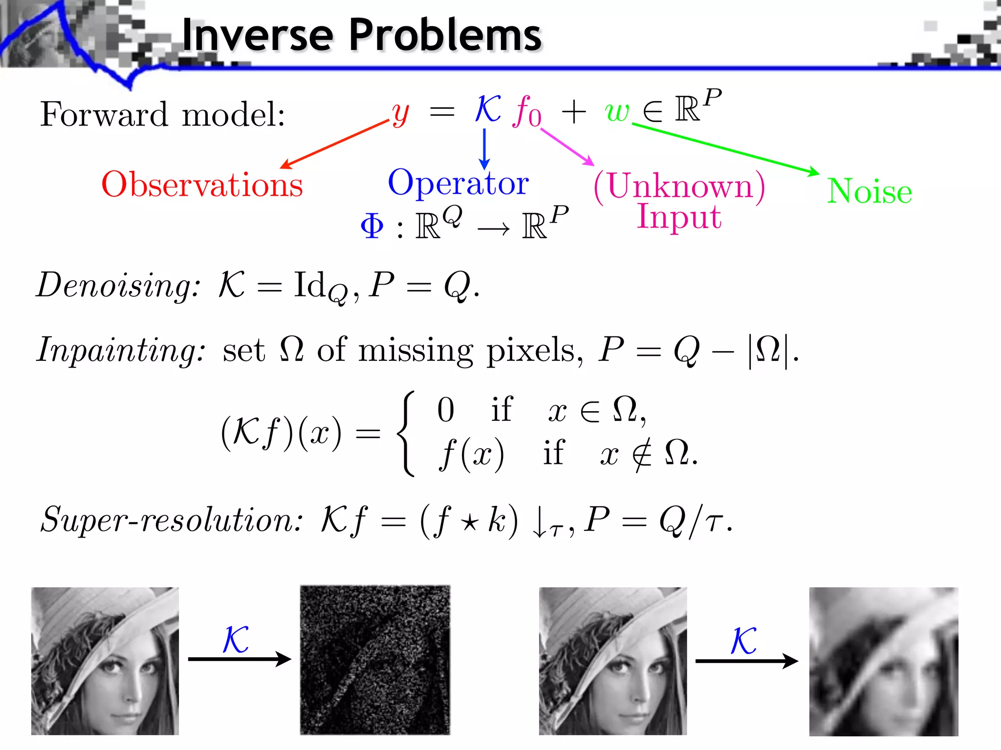
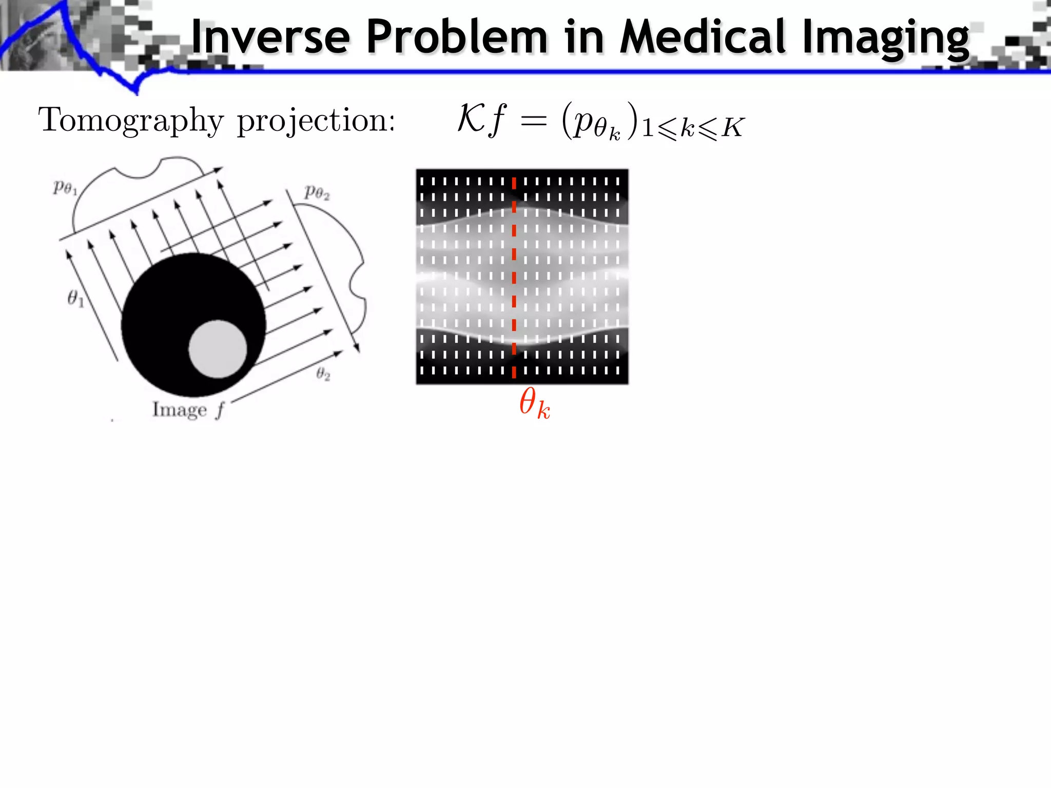
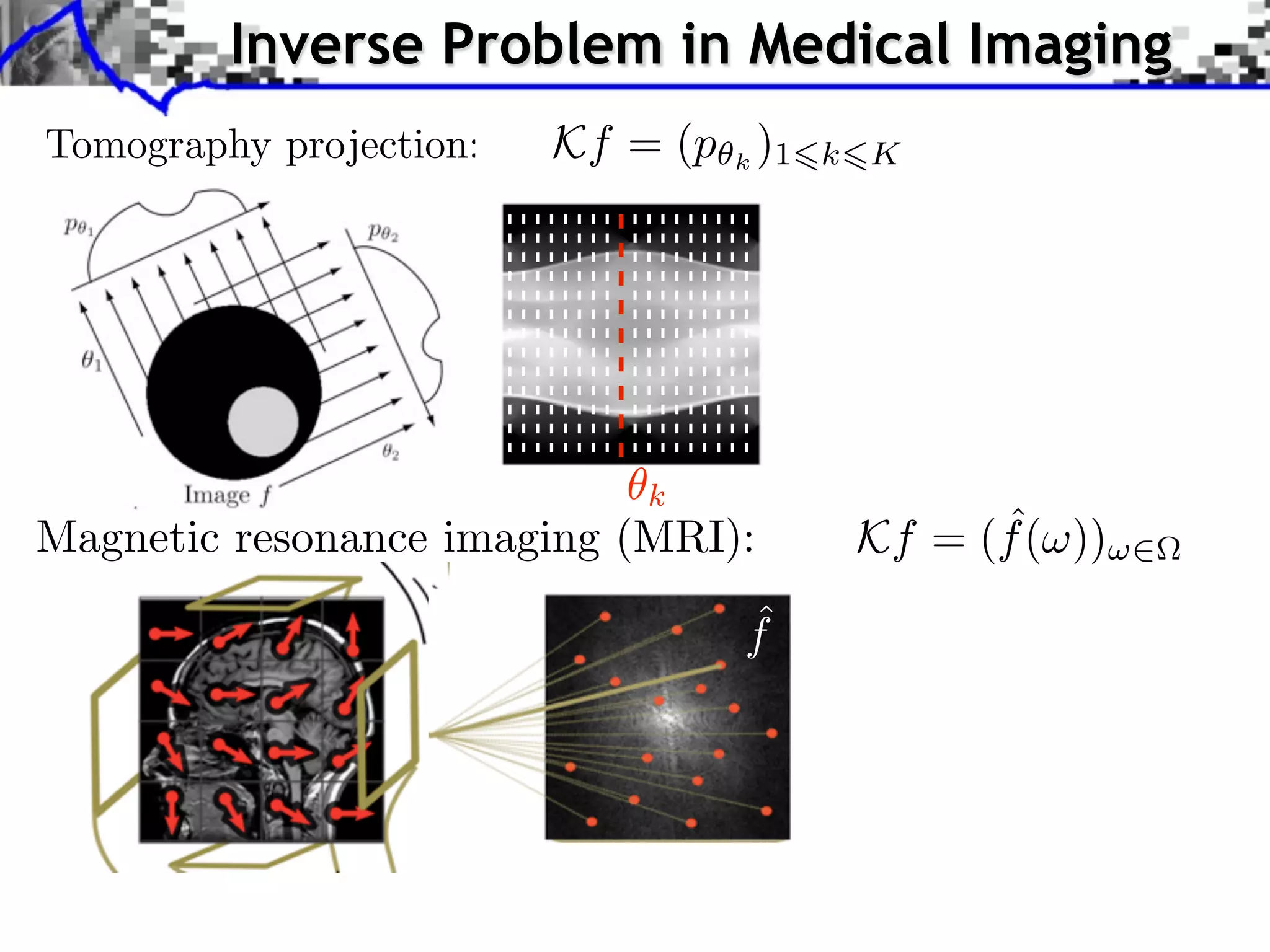
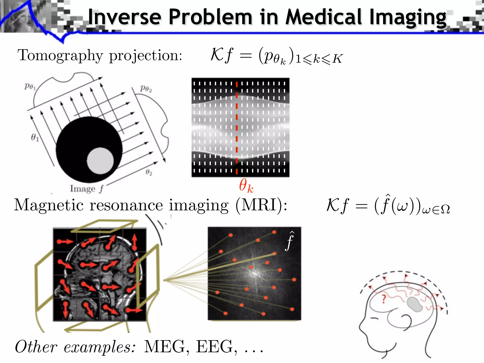
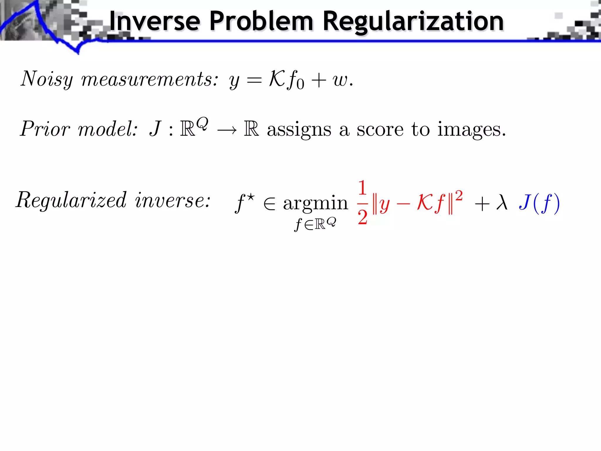
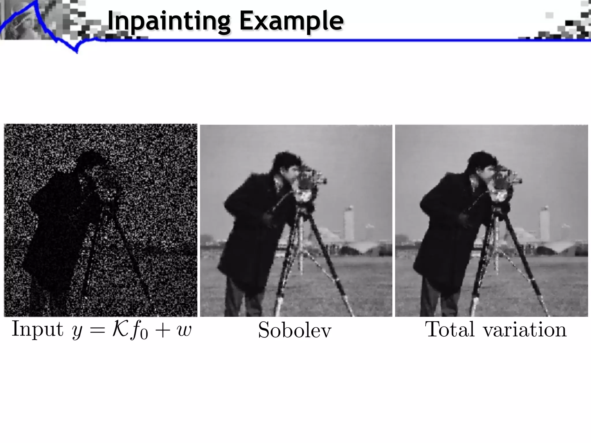
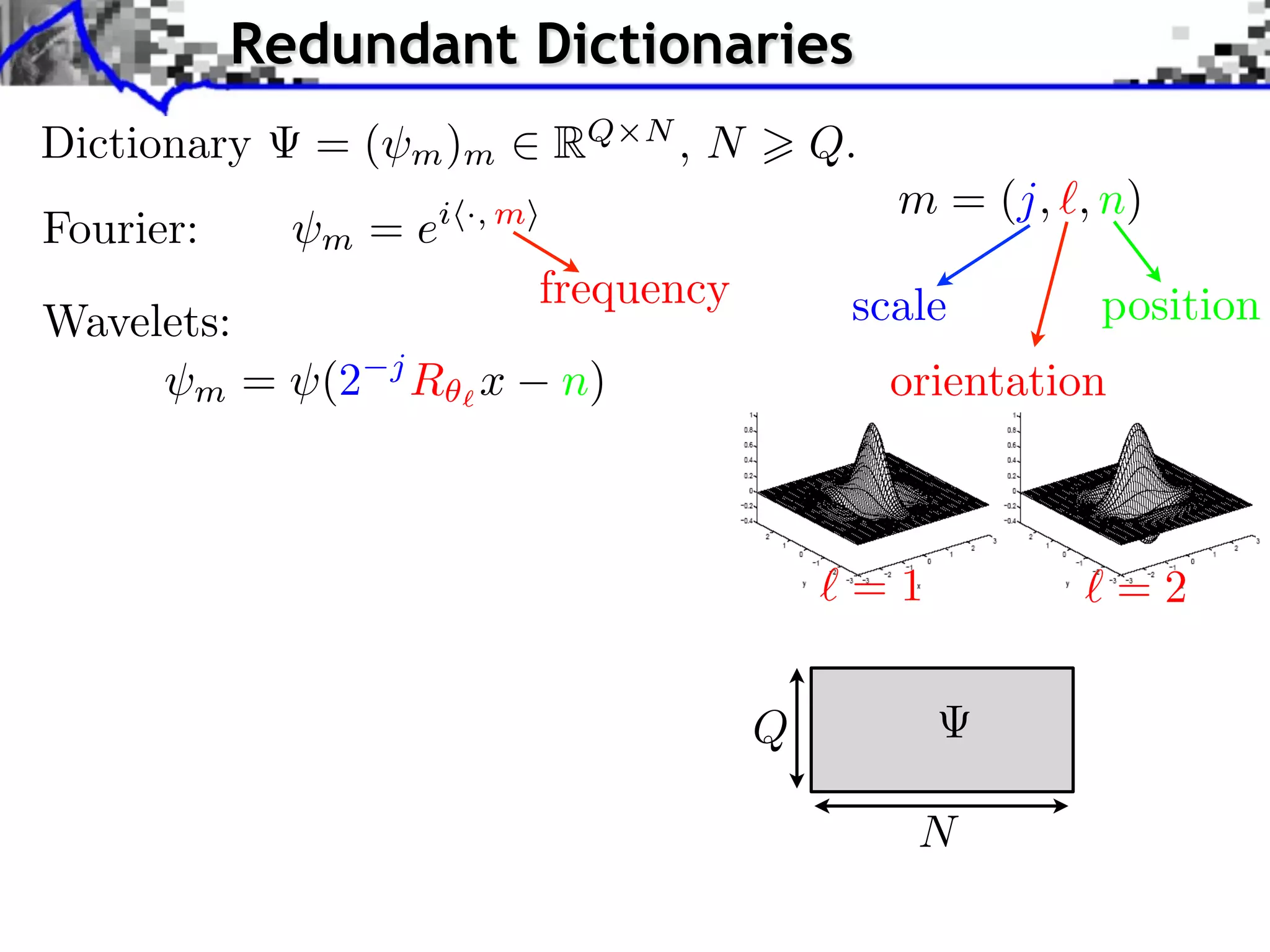
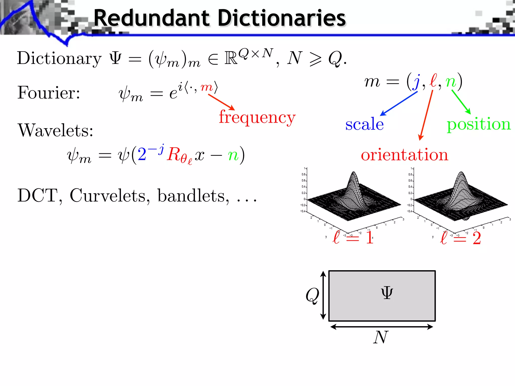
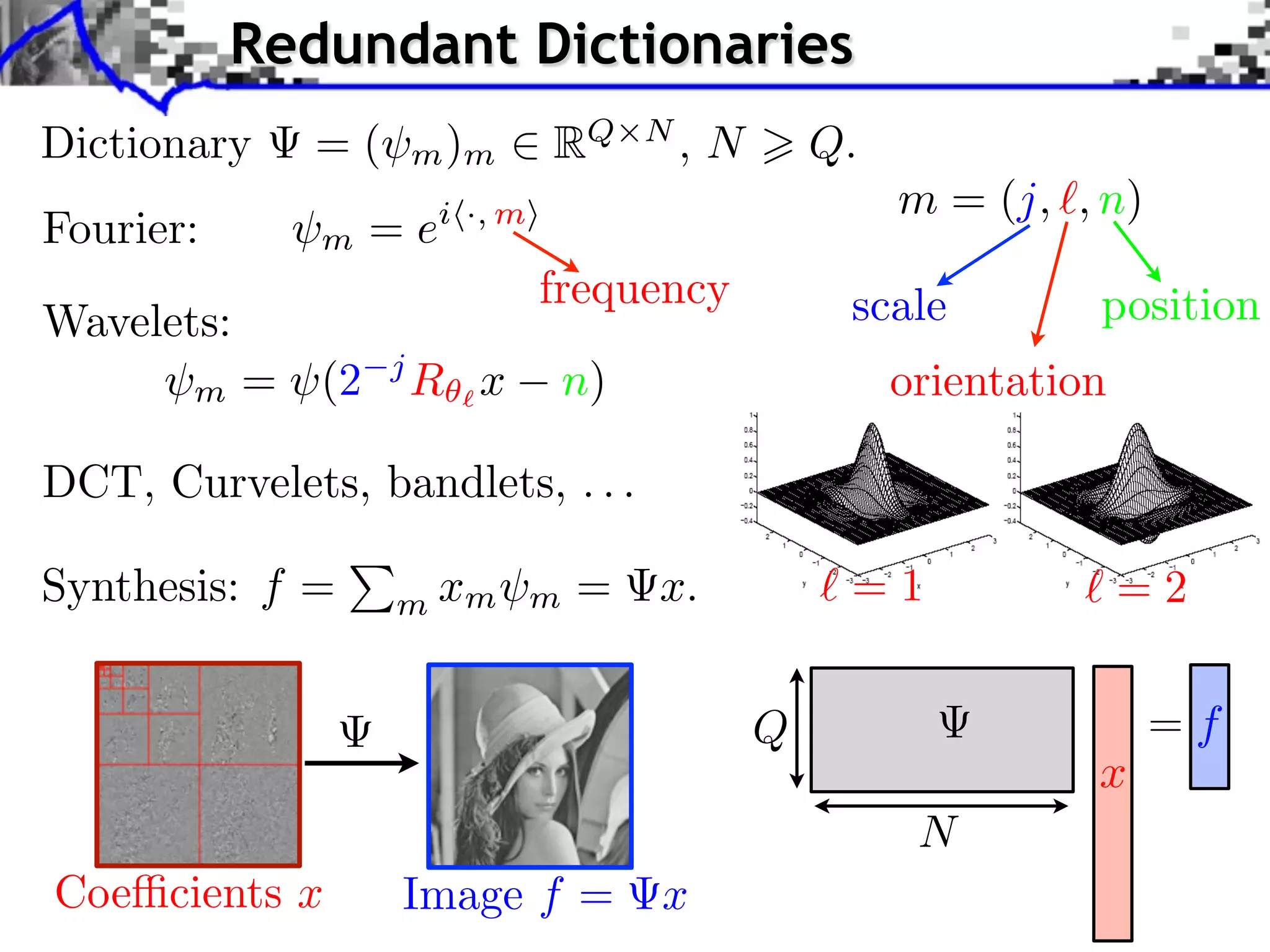
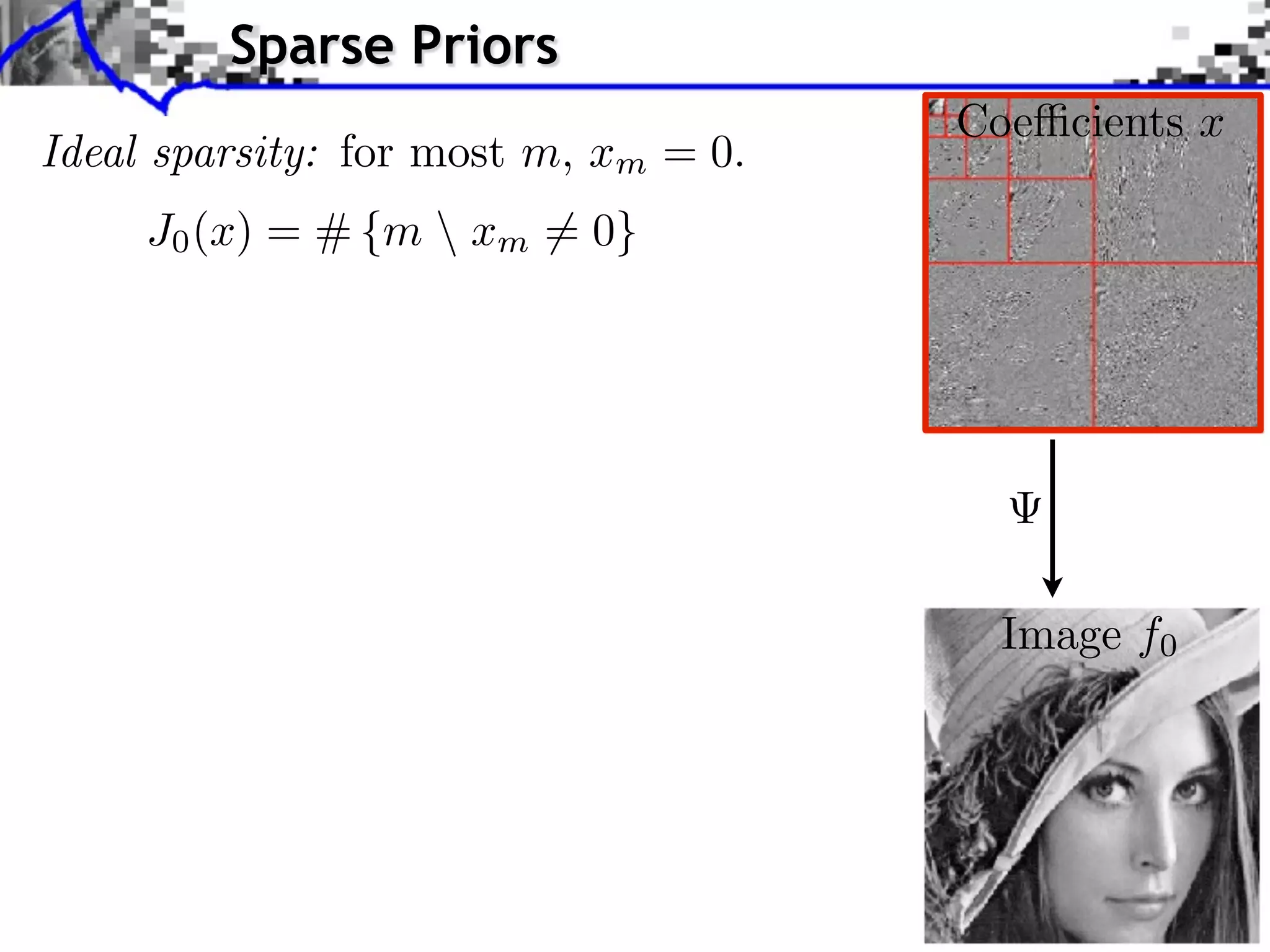
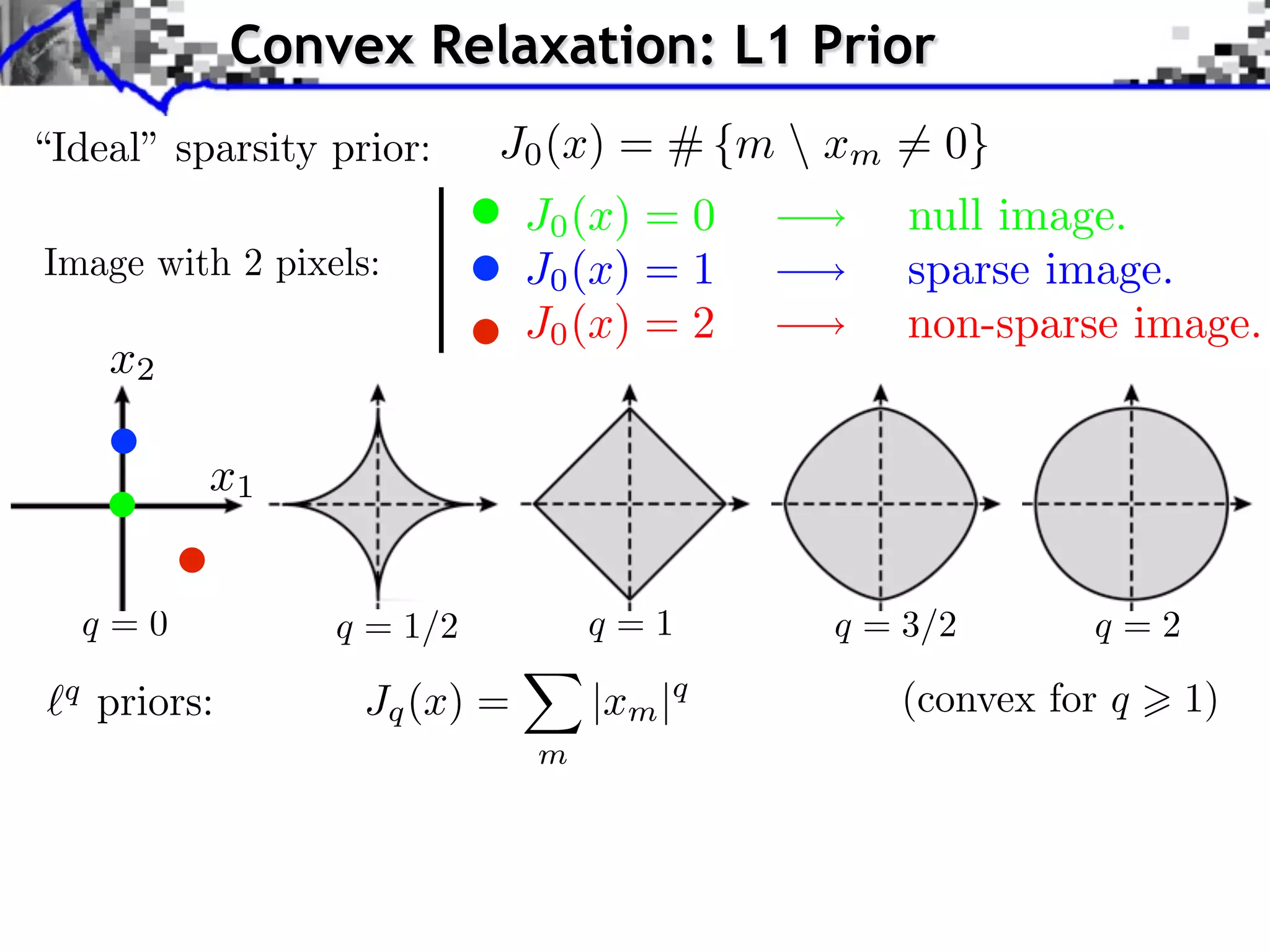
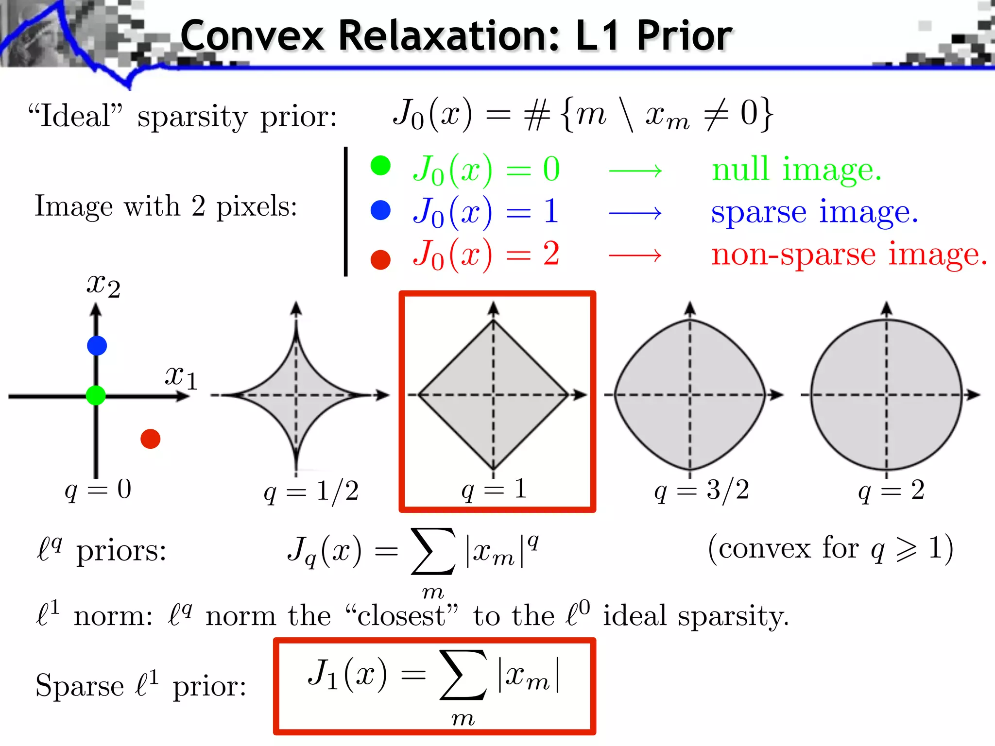
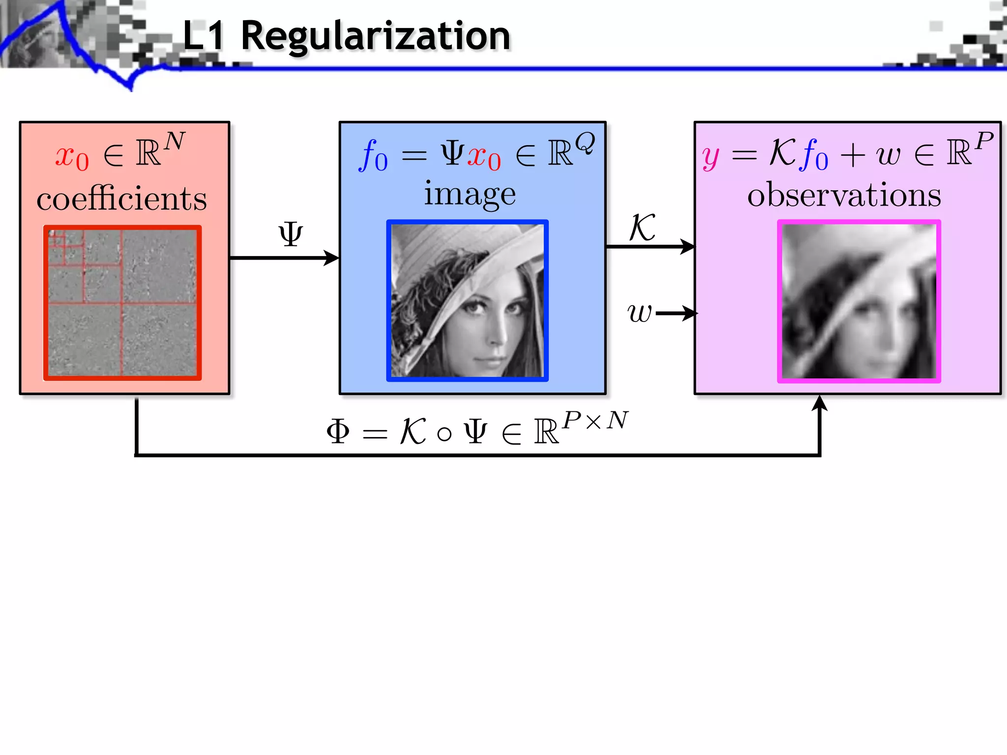
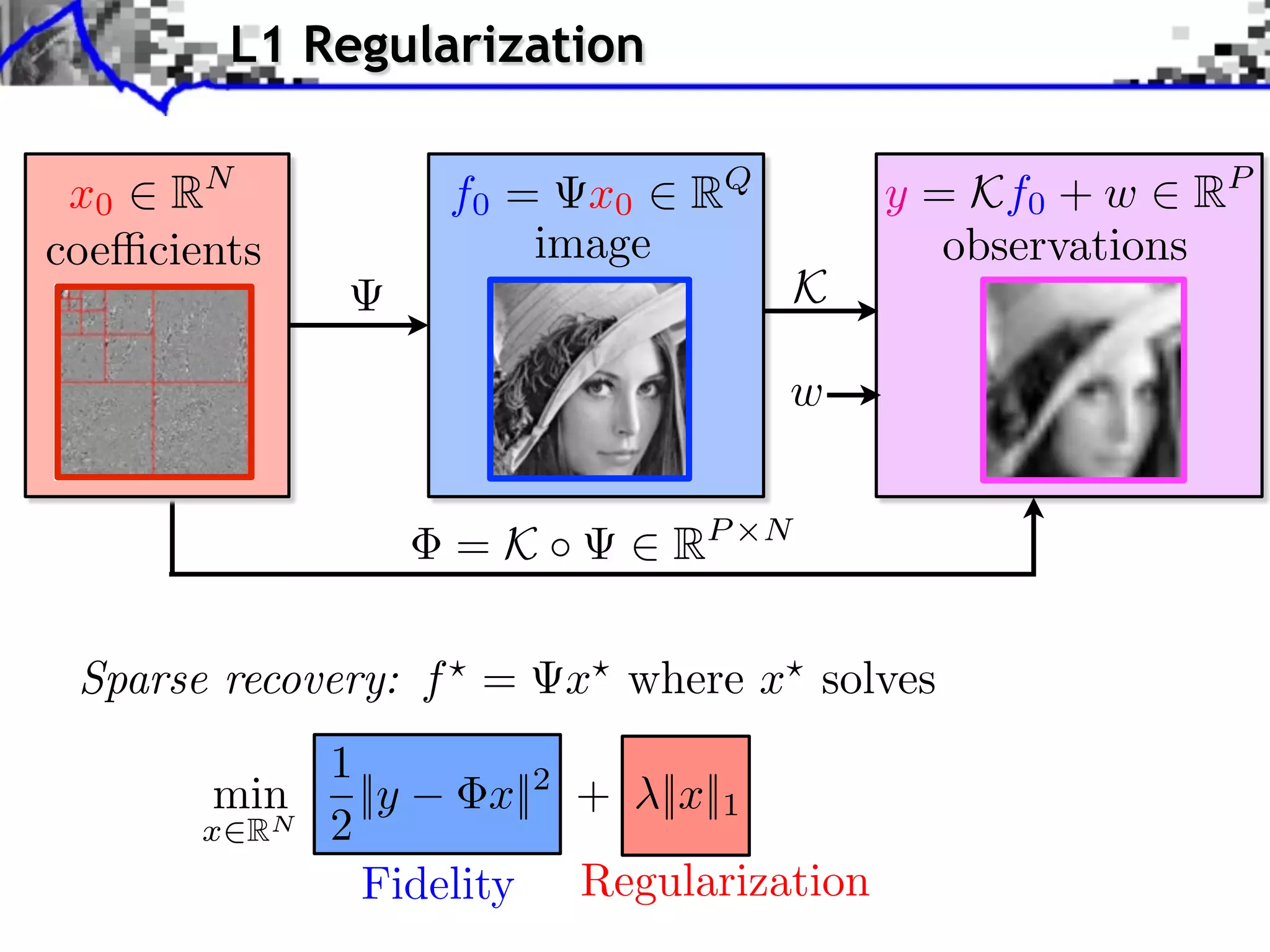
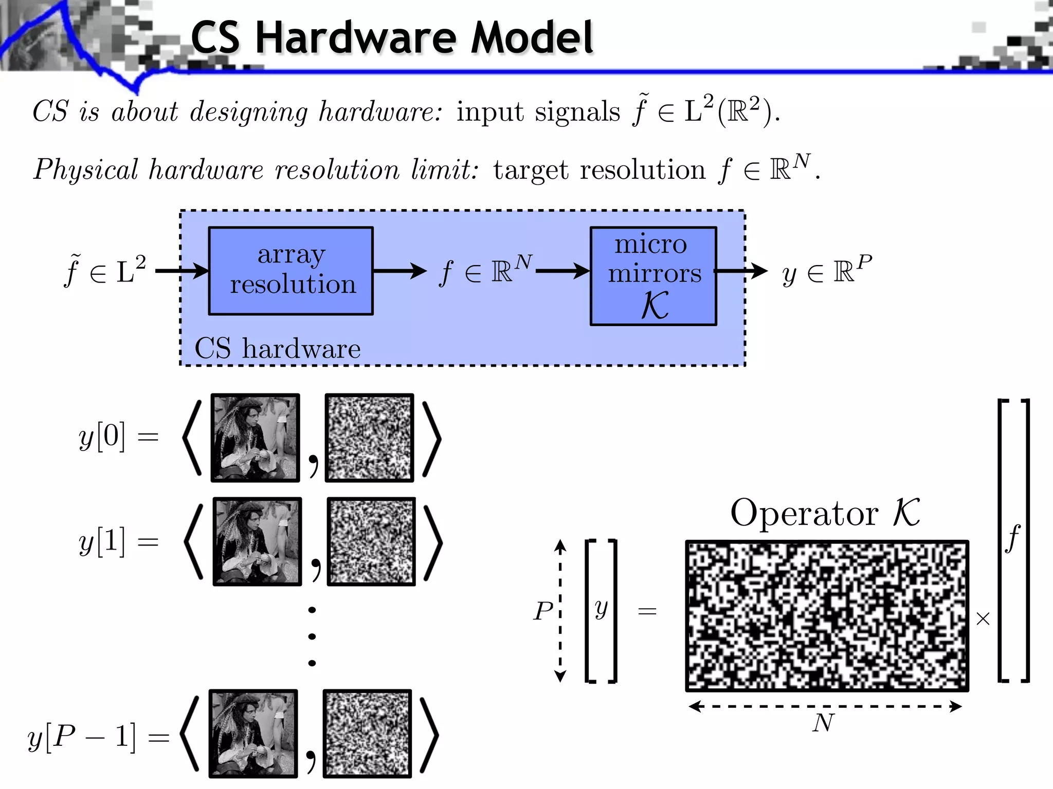
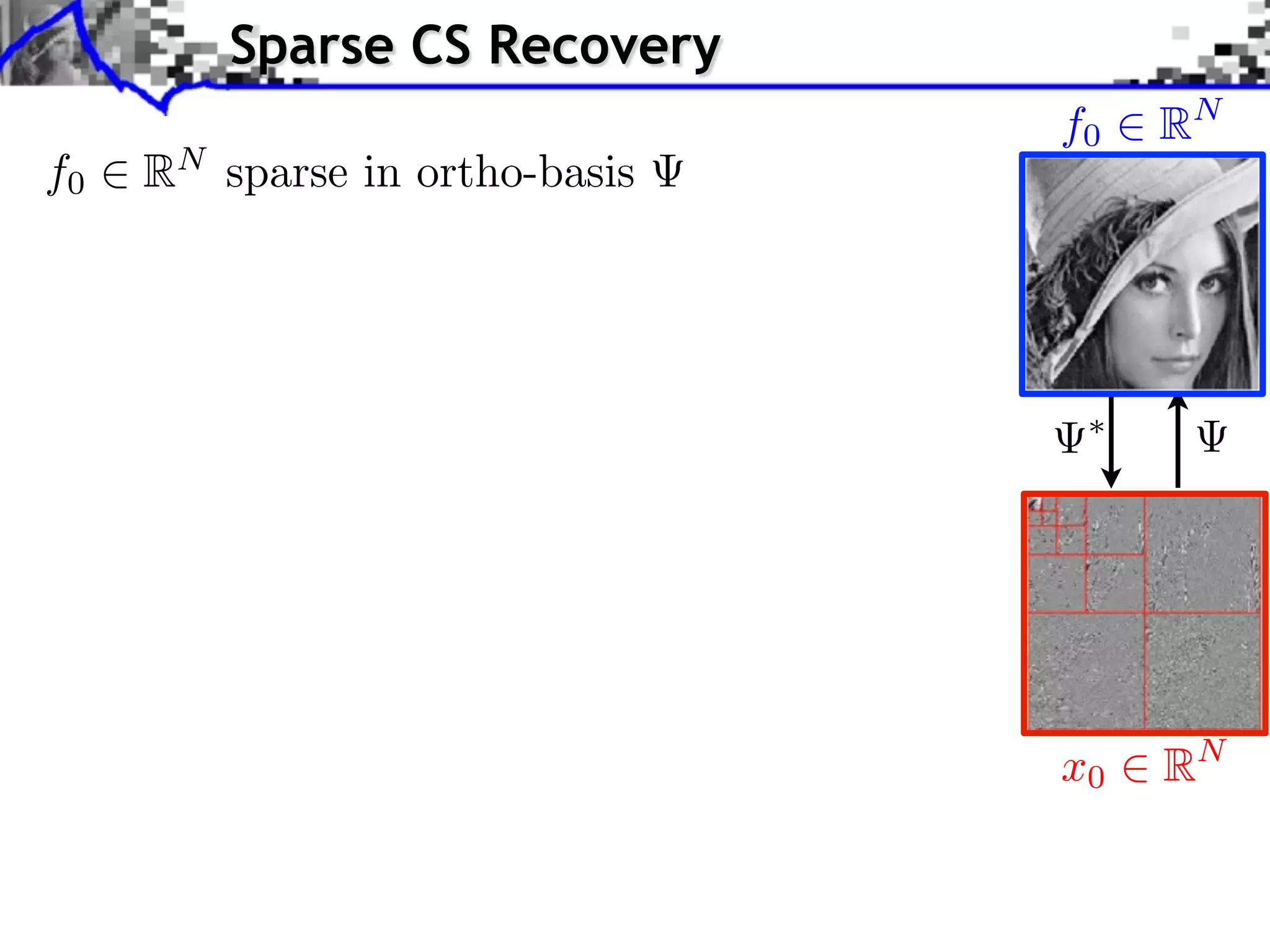
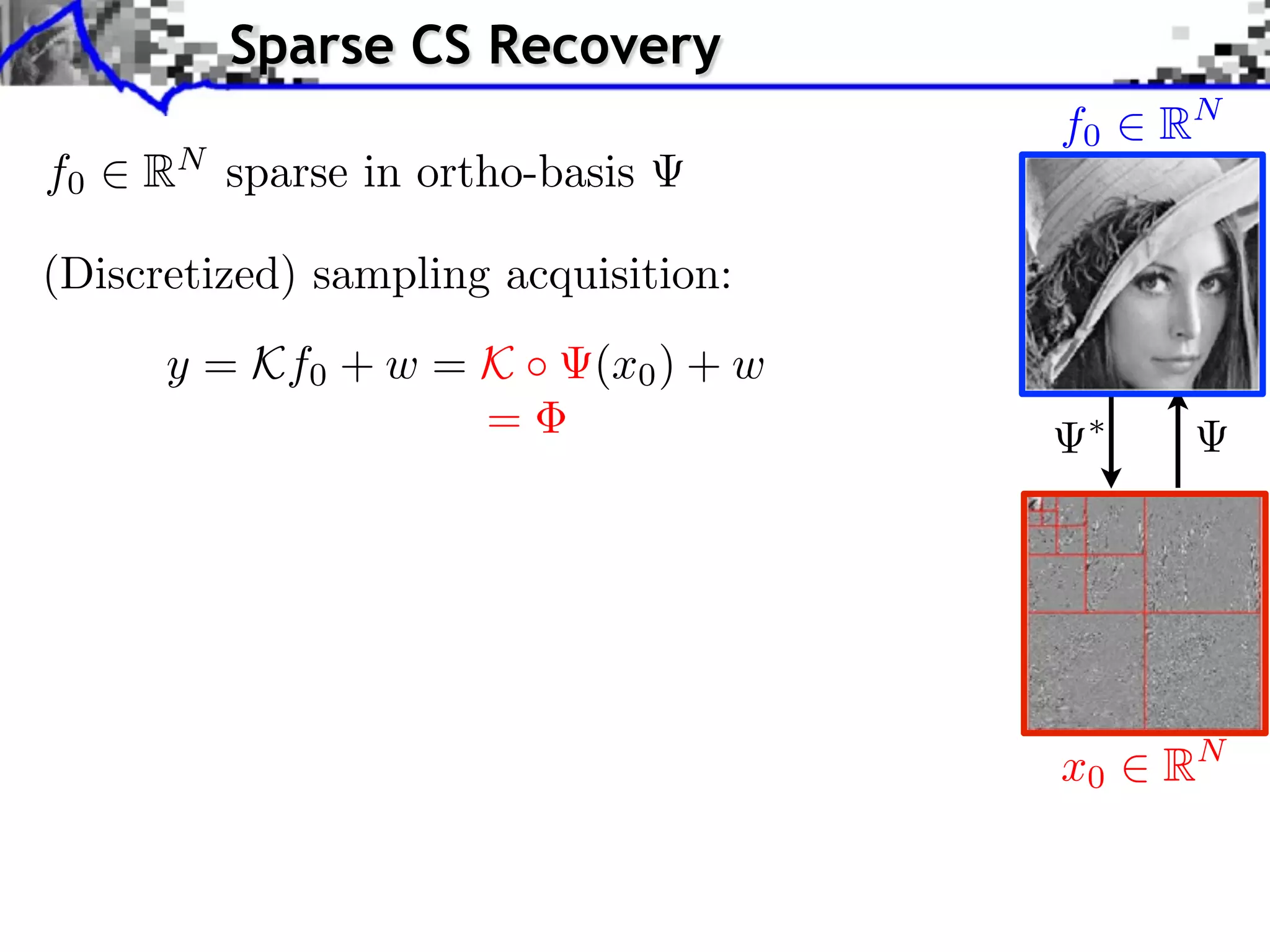
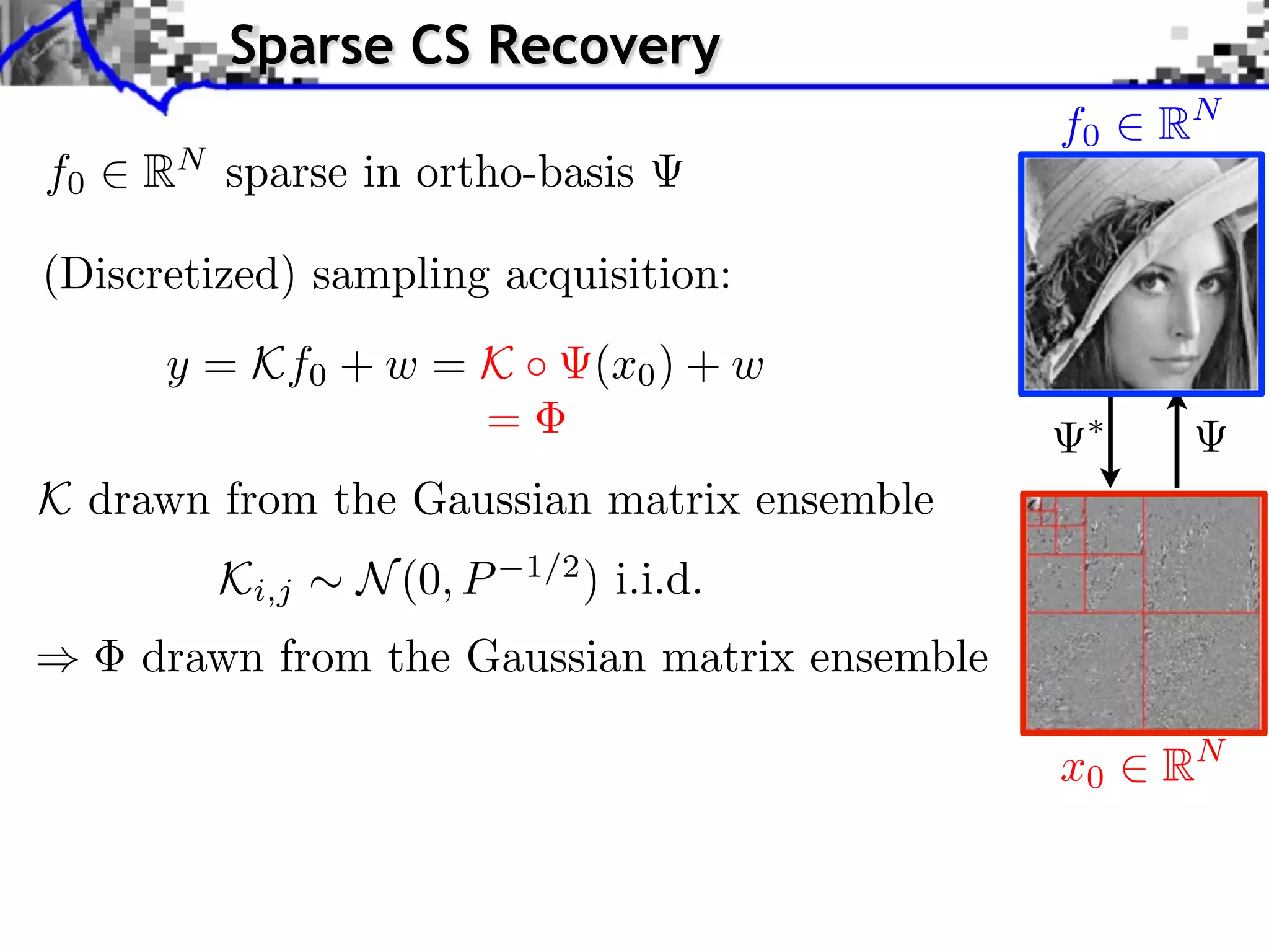
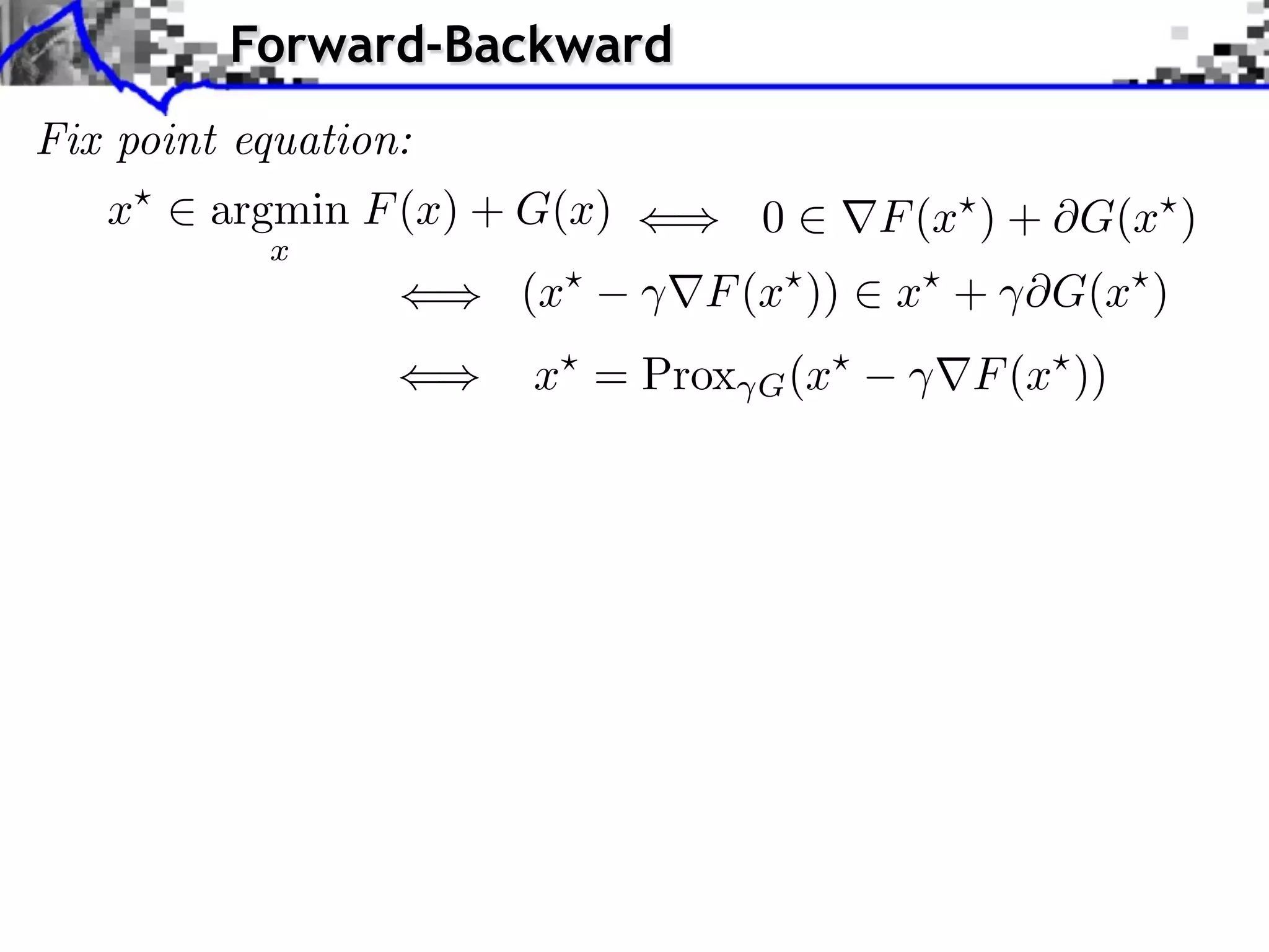
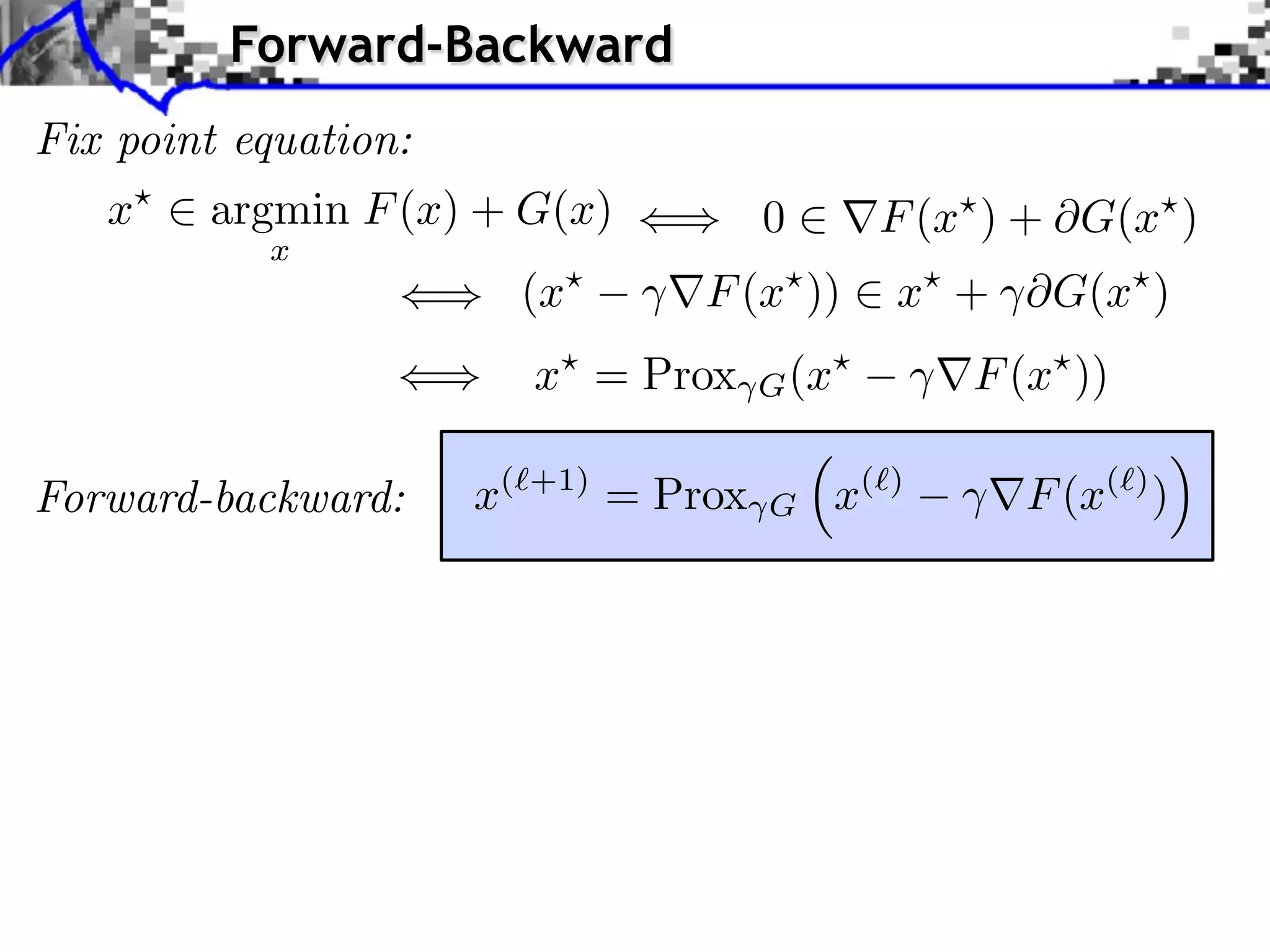
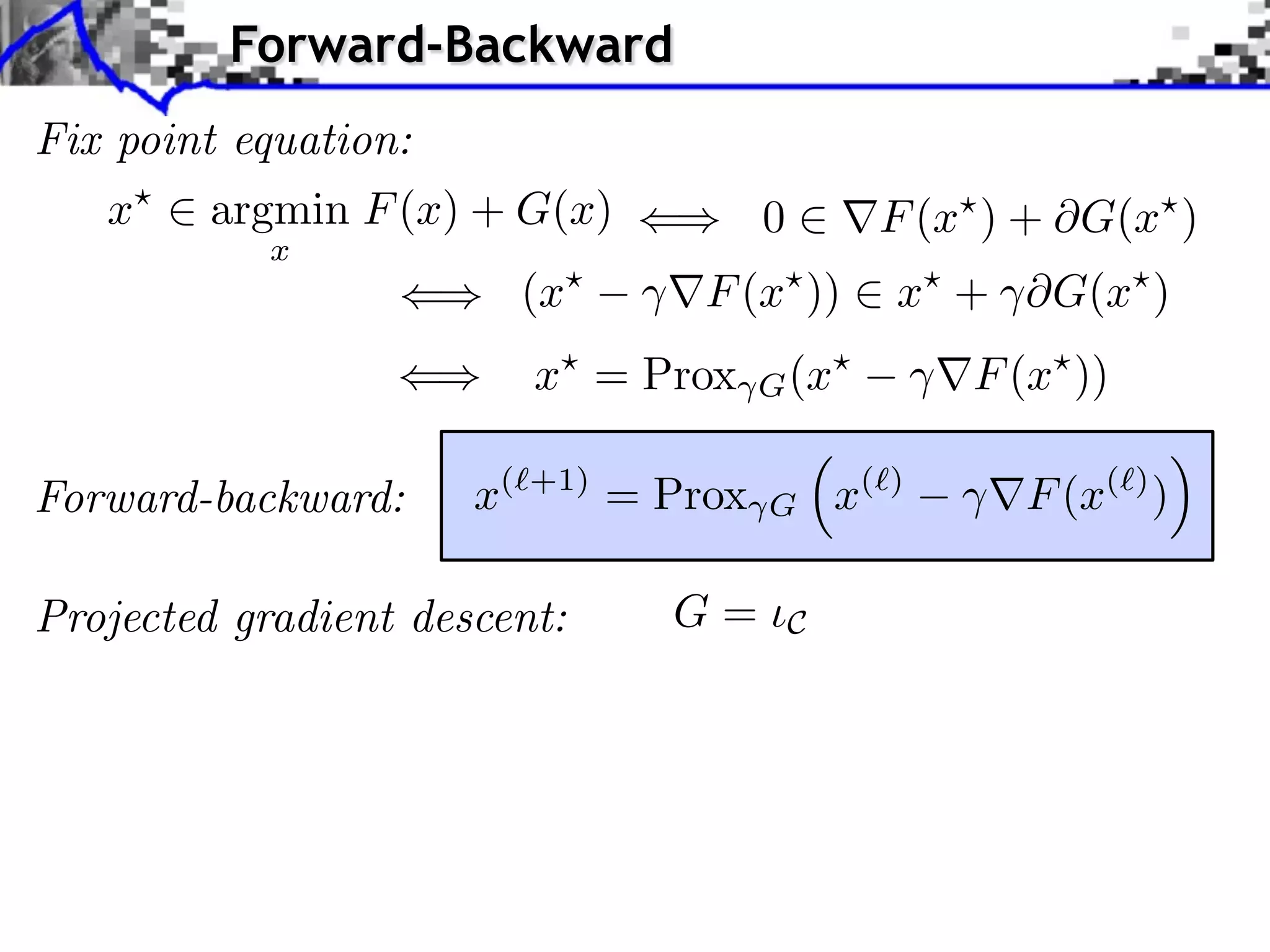
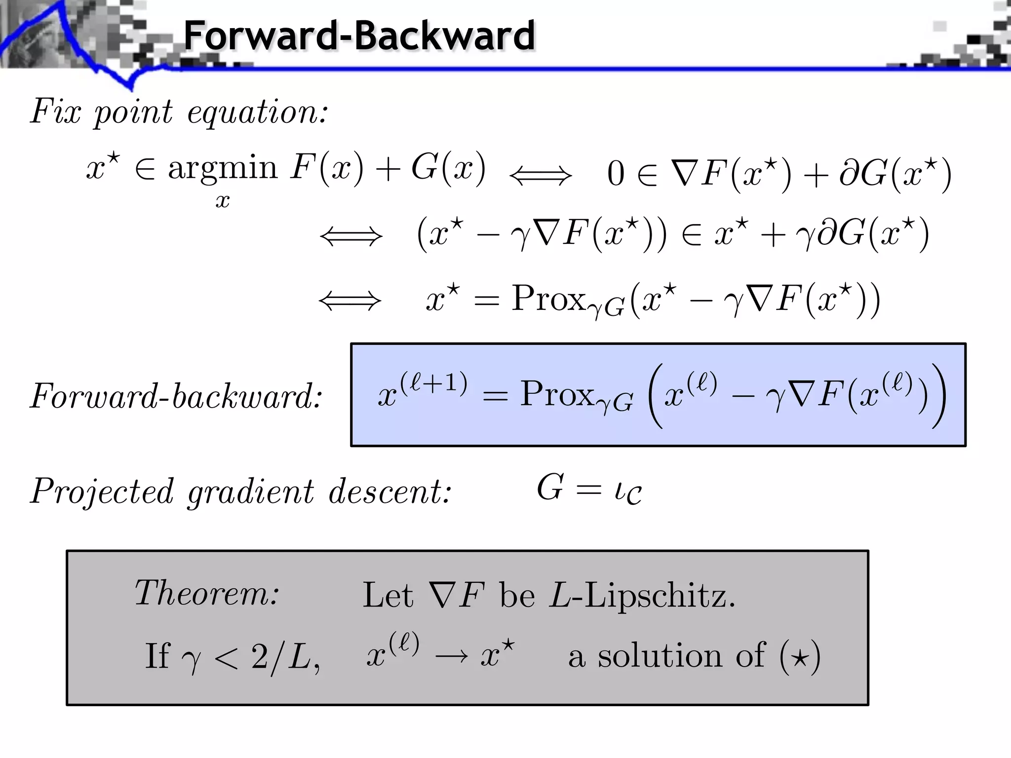
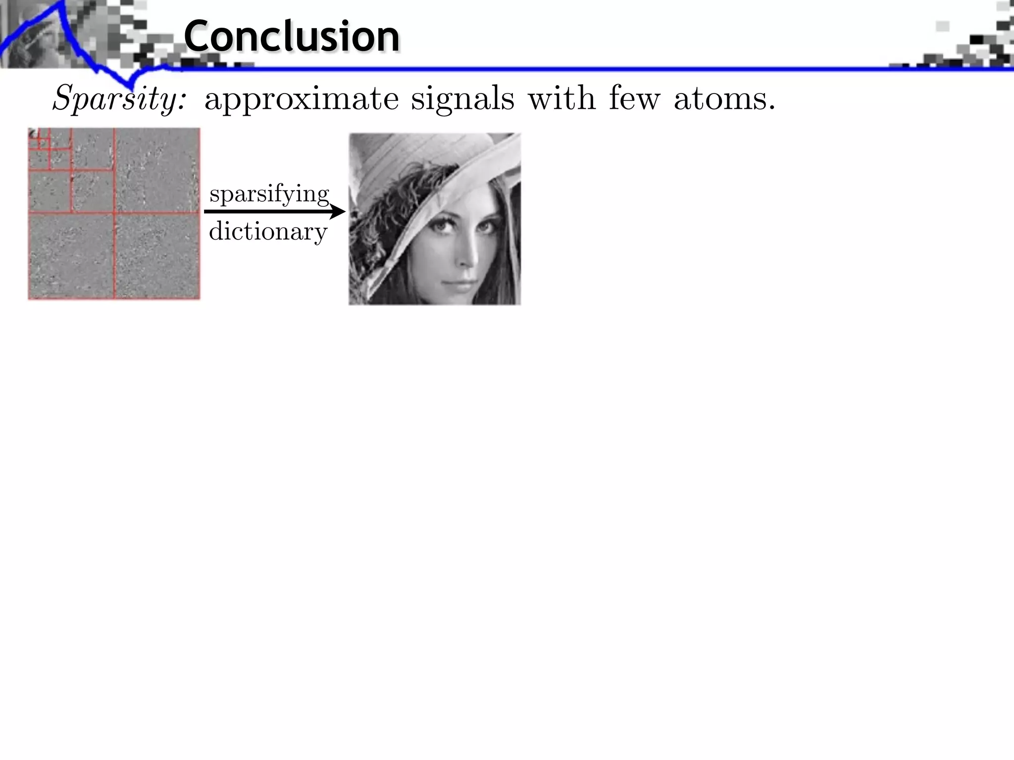
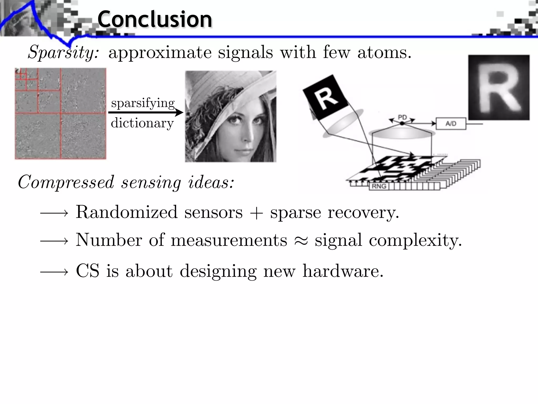
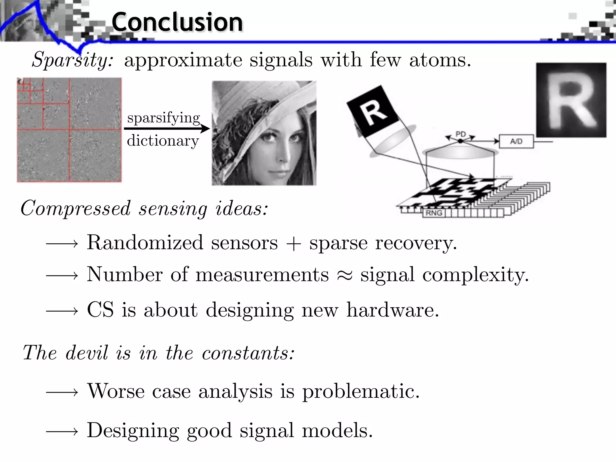
The document discusses inverse problems in the context of sparse synthesis regularization and compressed sensing, outlining key concepts such as theoretical recovery guarantees, data fidelity, and regularization methods. It provides an overview of various techniques for denoising, inpainting, super-resolution, and image separation, alongside the mathematical frameworks and algorithms involved. Additionally, it touches on convex optimization strategies and the use of redundant dictionaries for sparse approximations in image processing.