Download as PDF, PPTX


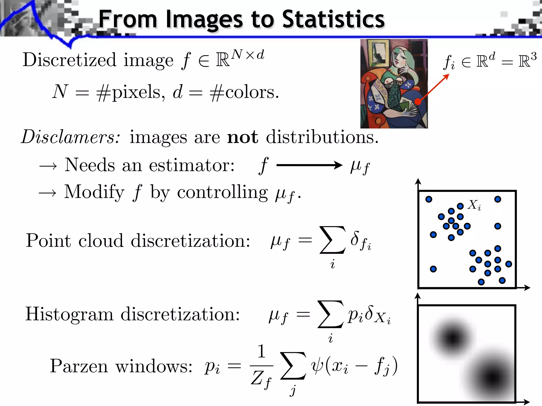
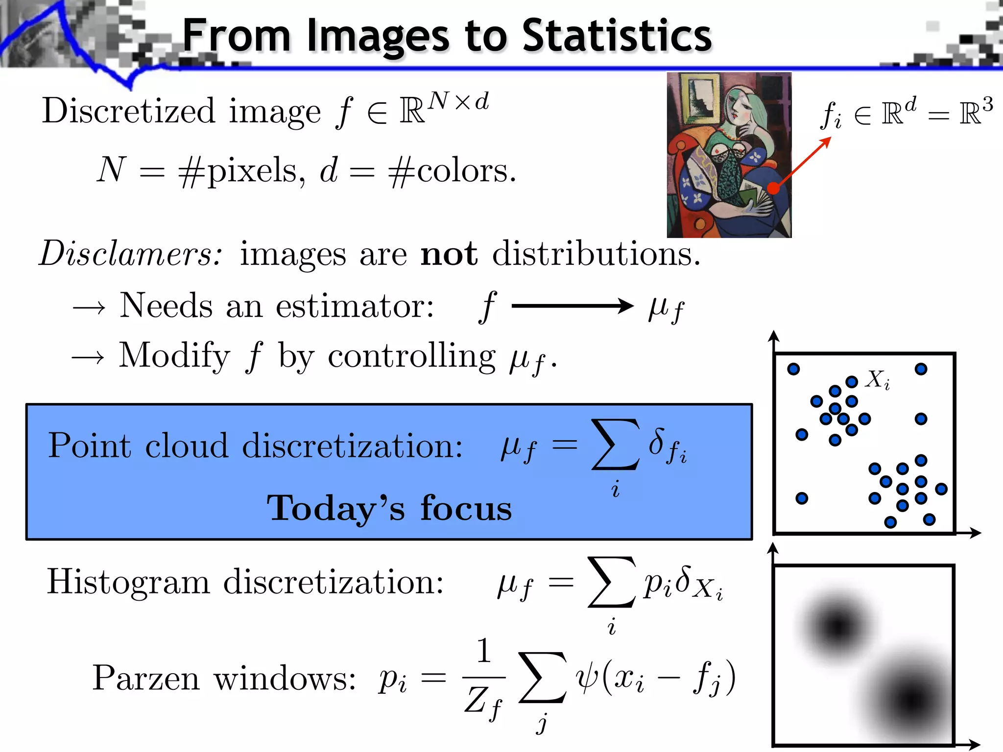
![Approximate Sliced Distance
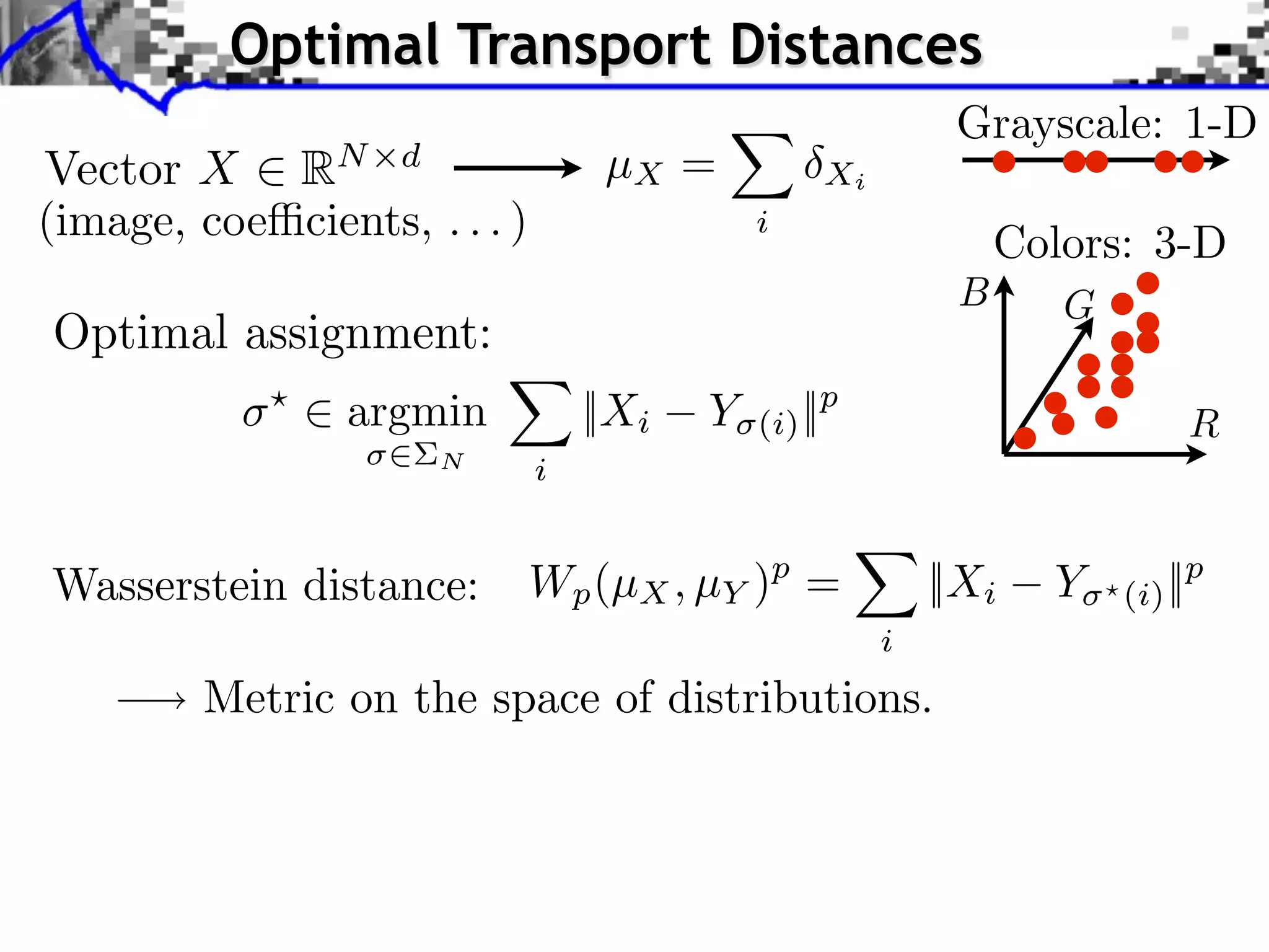
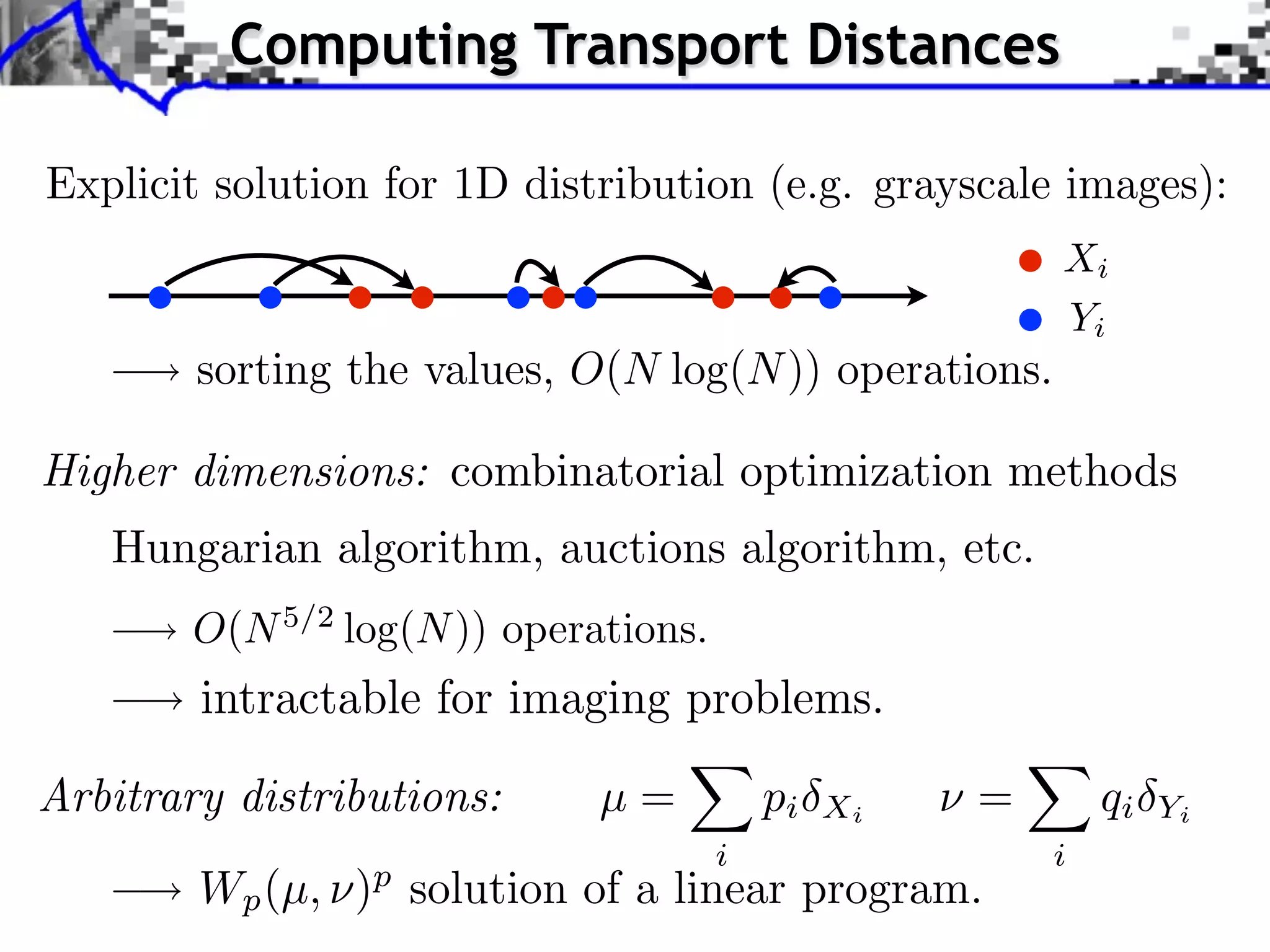
Key idea: replace transport in Rd by series of 1D transport.
Xi
[Rabin, Peyr´, Delon & Bernot 2010]
e
Projected point cloud: X = { Xi , ⇥}i .
Xi ,](https://image.slidesharecdn.com/2012-06-21-orsay-121213050319-phpapp01/75/Optimal-Transport-in-Imaging-Sciences-22-2048.jpg)
![Approximate Sliced Distance
Key idea: replace transport in Rd by series of 1D transport.
Xi
[Rabin, Peyr´, Delon & Bernot 2010]
e
Projected point cloud: X = { Xi , ⇥}i .
Xi ,
Sliced Wasserstein distance: (p = 2)
SW (µX , µY )2 = W (µX , µY )2 d
|| ||=1](https://image.slidesharecdn.com/2012-06-21-orsay-121213050319-phpapp01/75/Optimal-Transport-in-Imaging-Sciences-23-2048.jpg)
![Approximate Sliced Distance
Key idea: replace transport in Rd by series of 1D transport.
Xi
[Rabin, Peyr´, Delon & Bernot 2010]
e
Projected point cloud: X = { Xi , ⇥}i .
Xi ,
Sliced Wasserstein distance: (p = 2)
SW (µX , µY )2 = W (µX , µY )2 d
|| ||=1
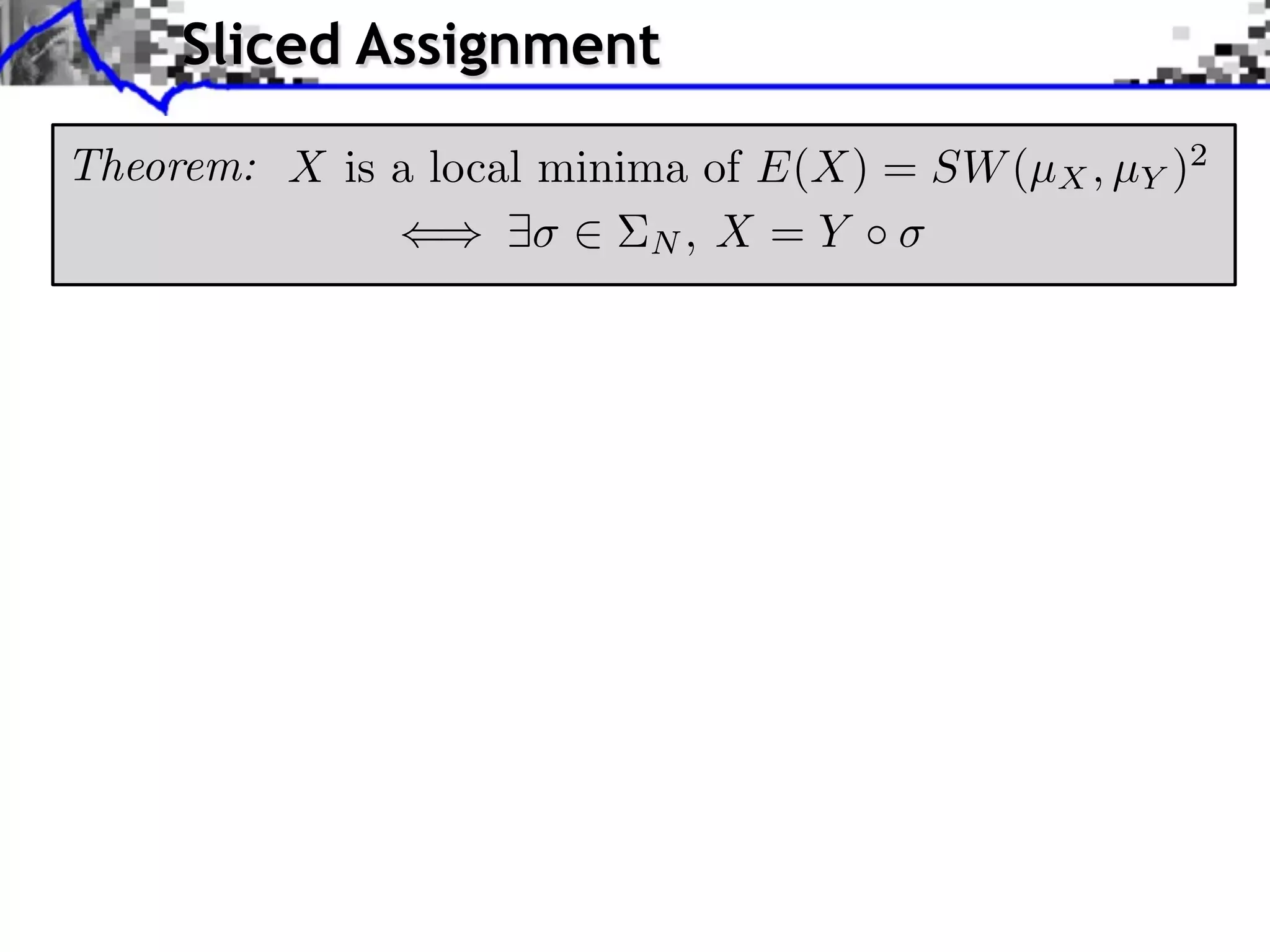
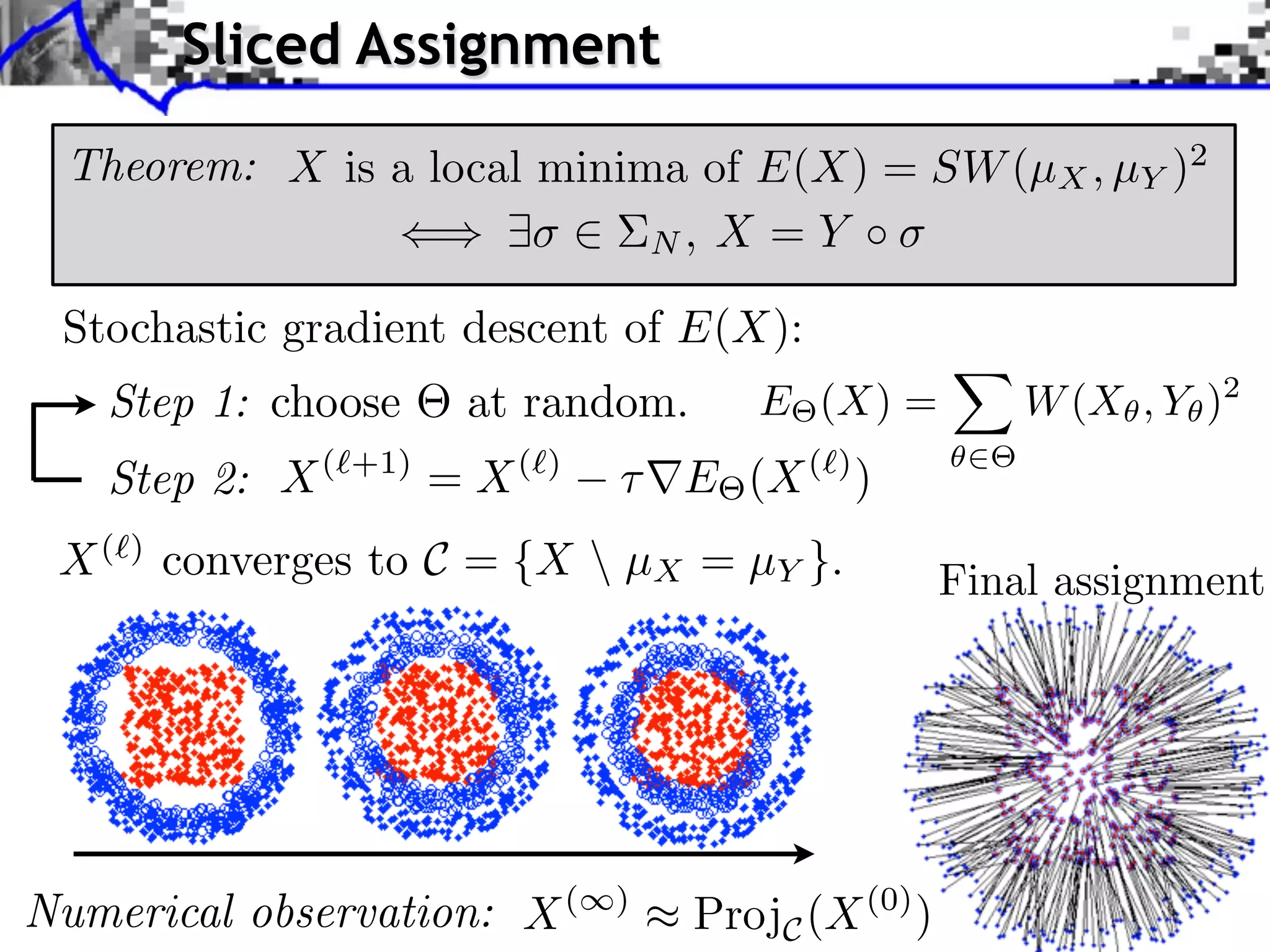
Theorem: E(X) = SW (µX , µY )2 is of class C 1 and
E(X) = Xi Y⇥ (i) , d .
where N are 1-D optimal assignents of X and Y .](https://image.slidesharecdn.com/2012-06-21-orsay-121213050319-phpapp01/75/Optimal-Transport-in-Imaging-Sciences-24-2048.jpg)
![Approximate Sliced Distance
Key idea: replace transport in Rd by series of 1D transport.
Xi
[Rabin, Peyr´, Delon & Bernot 2010]
e
Projected point cloud: X = { Xi , ⇥}i .
Xi ,
Sliced Wasserstein distance: (p = 2)
SW (µX , µY )2 = W (µX , µY )2 d
|| ||=1
Theorem: E(X) = SW (µX , µY )2 is of class C 1 and
E(X) = Xi Y⇥ (i) , d .
where N are 1-D optimal assignents of X and Y .
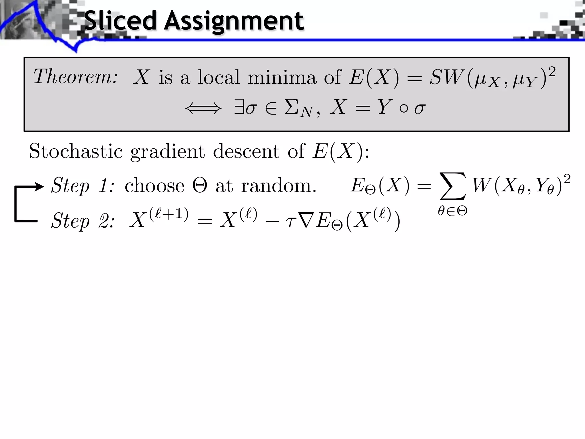
Possible to use SW in variational imaging problems.
Fast numerical scheme : use a few random .](https://image.slidesharecdn.com/2012-06-21-orsay-121213050319-phpapp01/75/Optimal-Transport-in-Imaging-Sciences-25-2048.jpg)

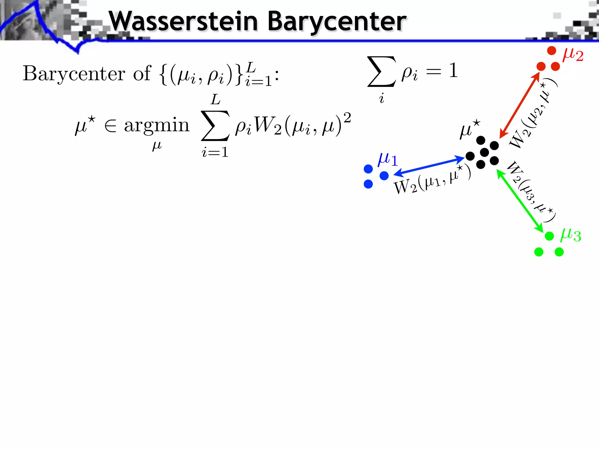
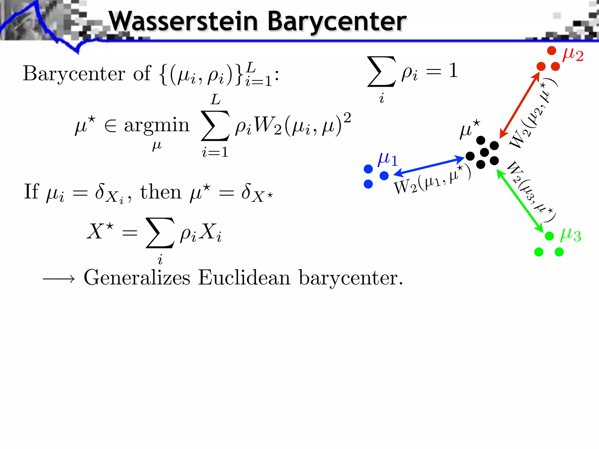
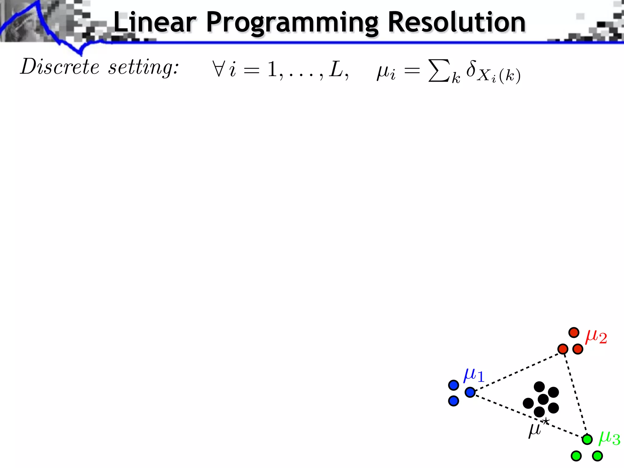
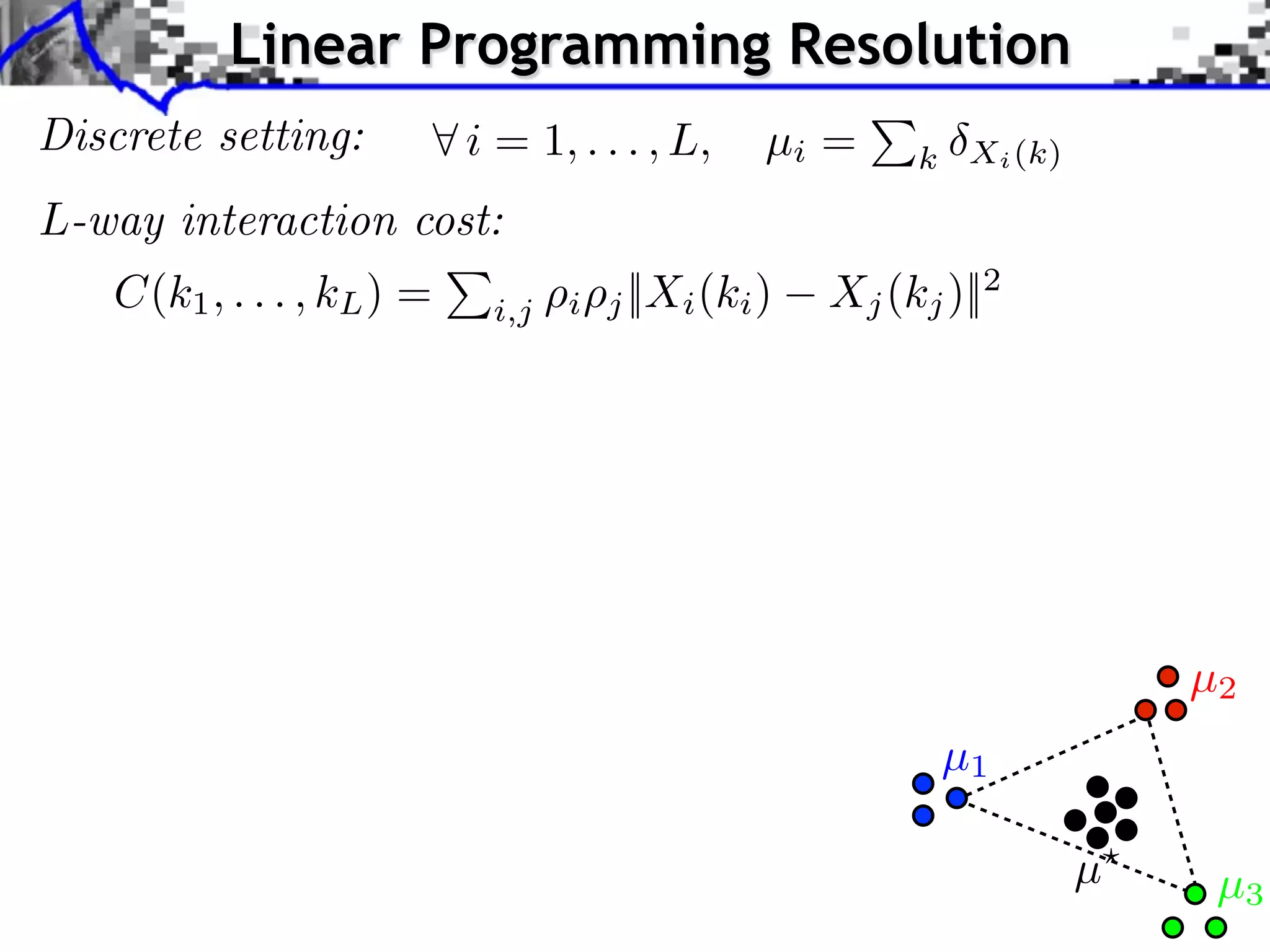
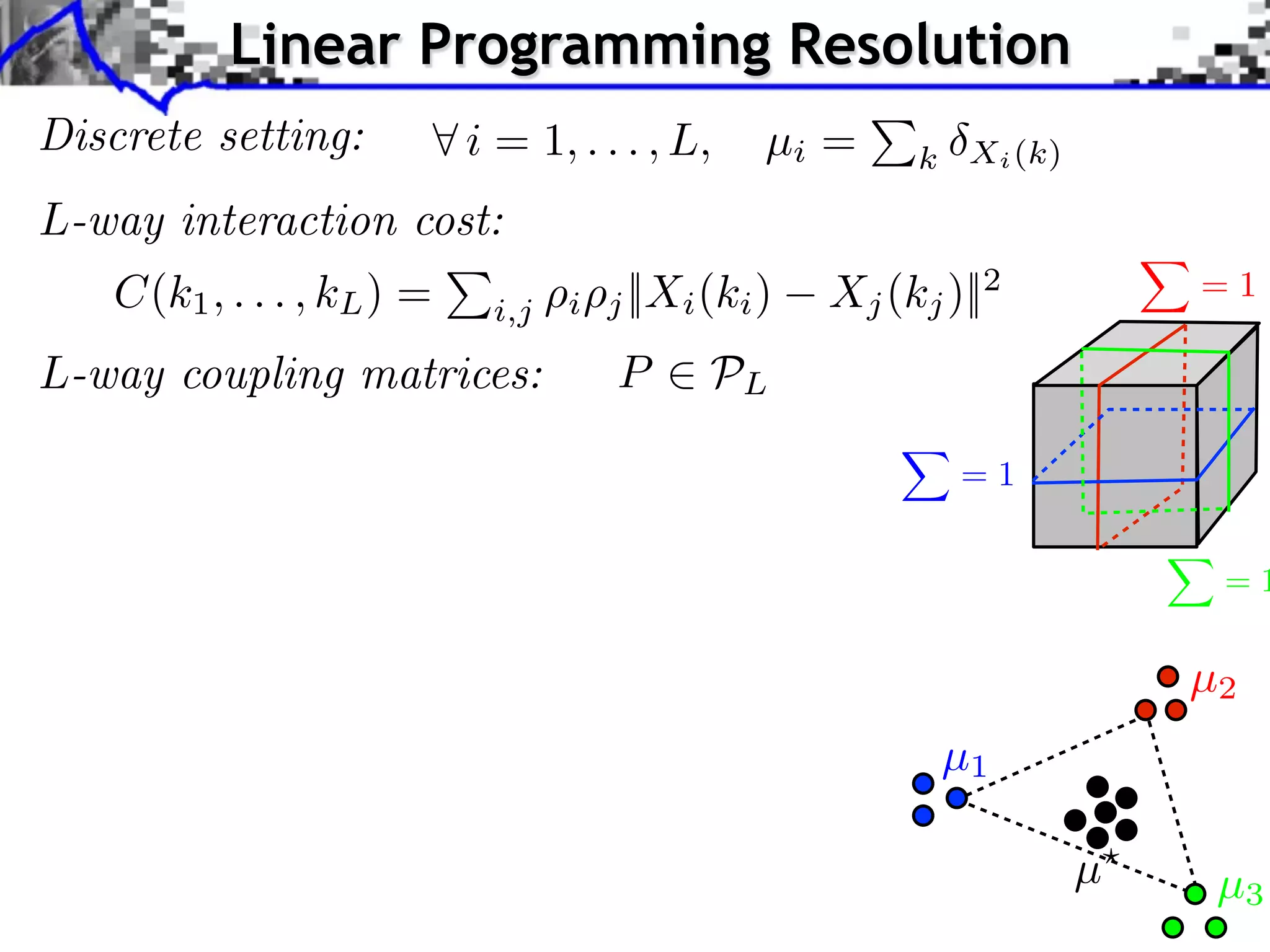
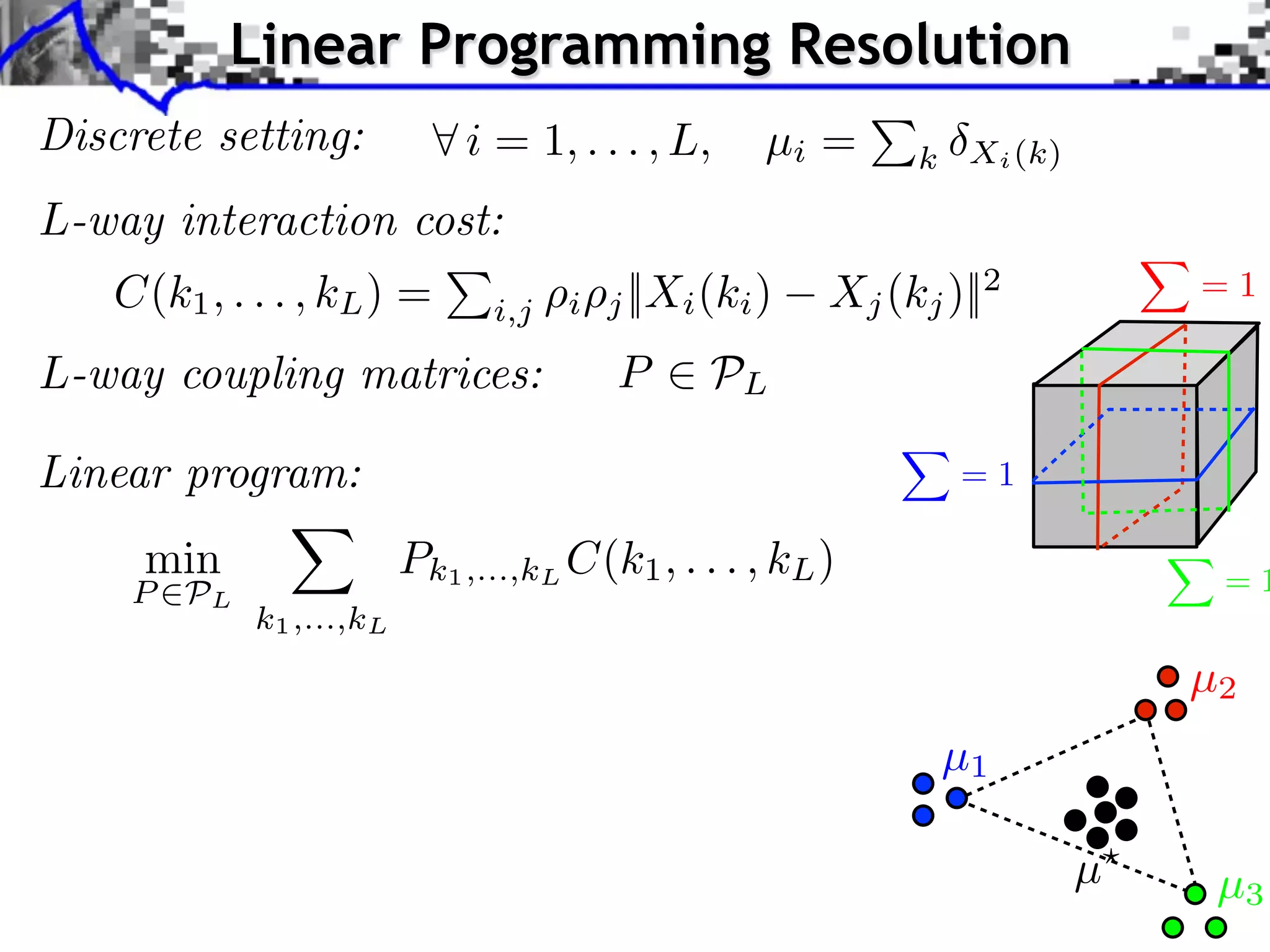
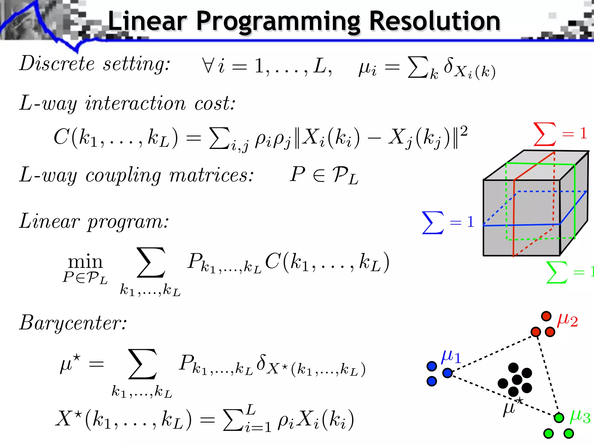
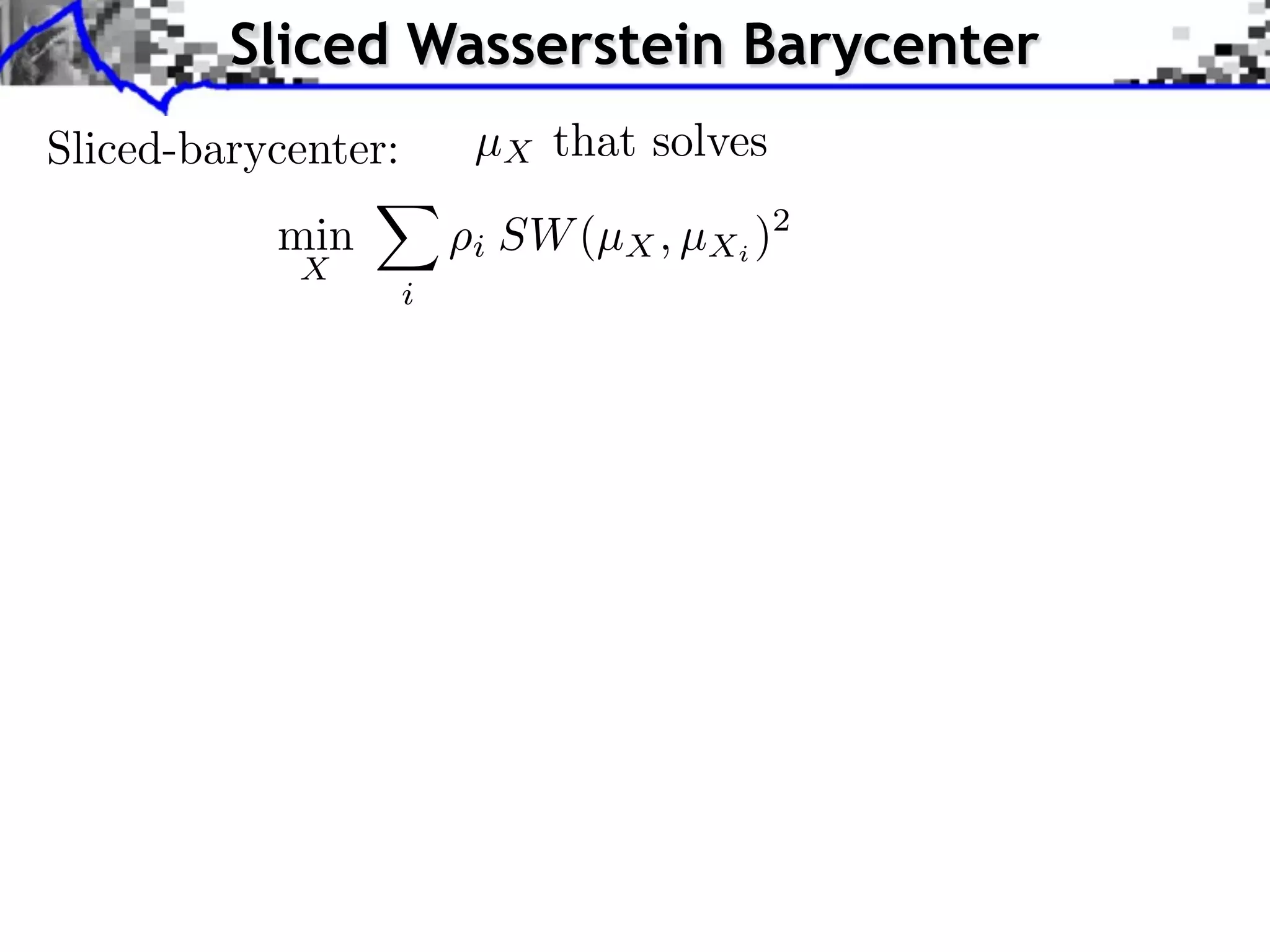
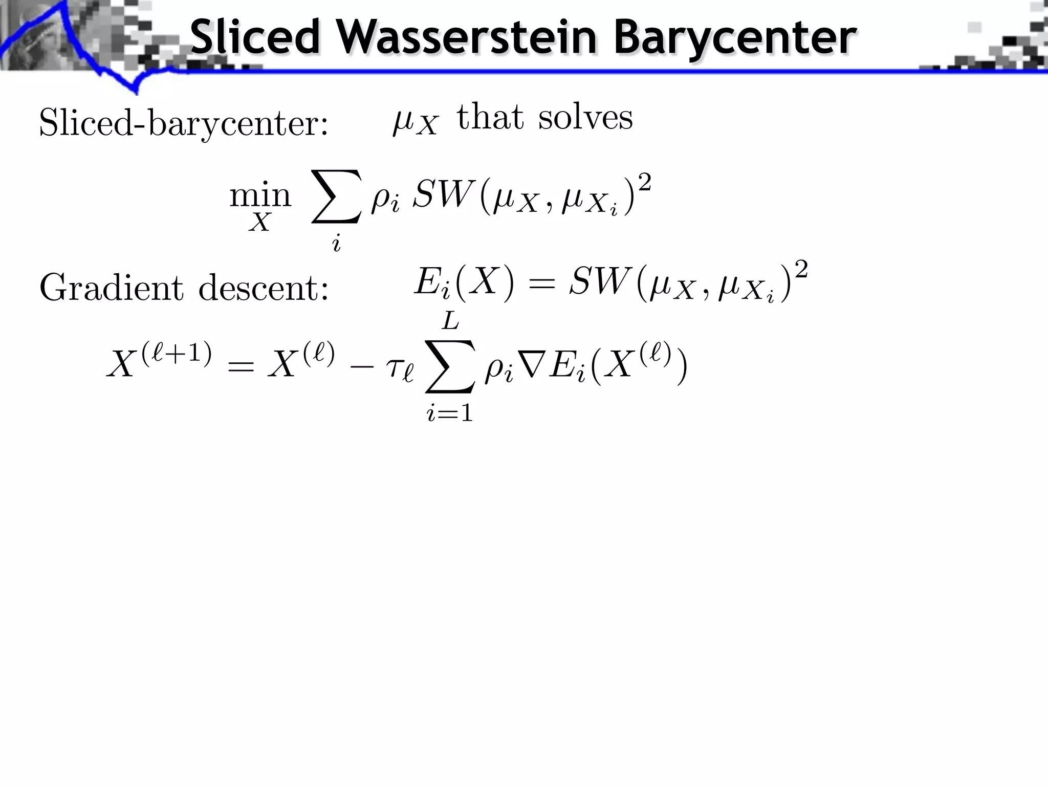
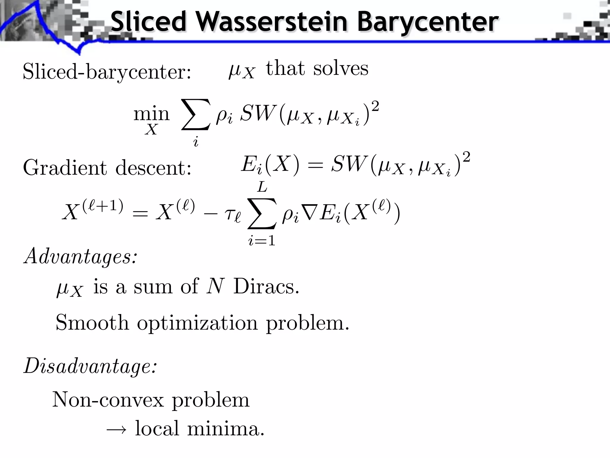
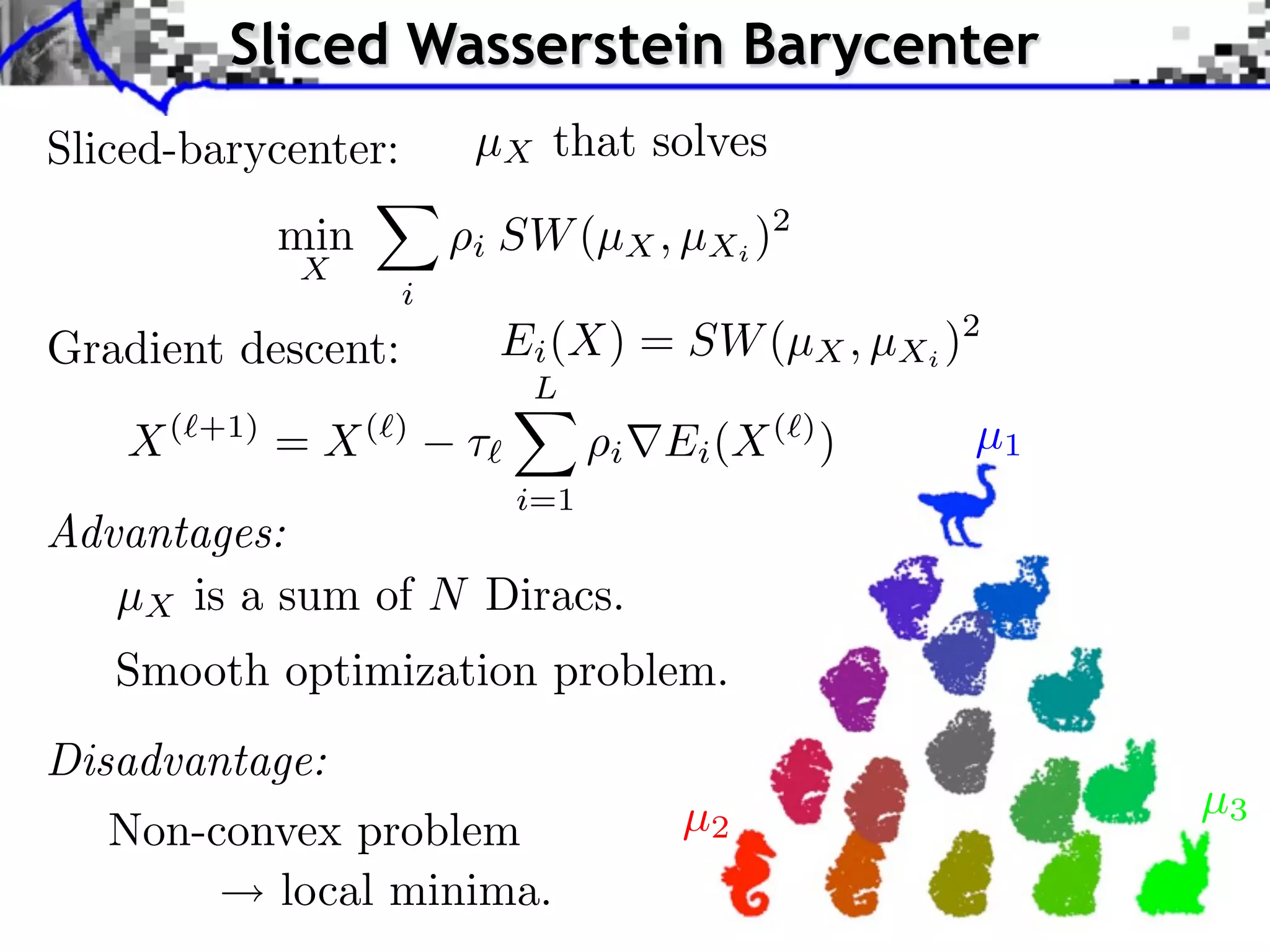
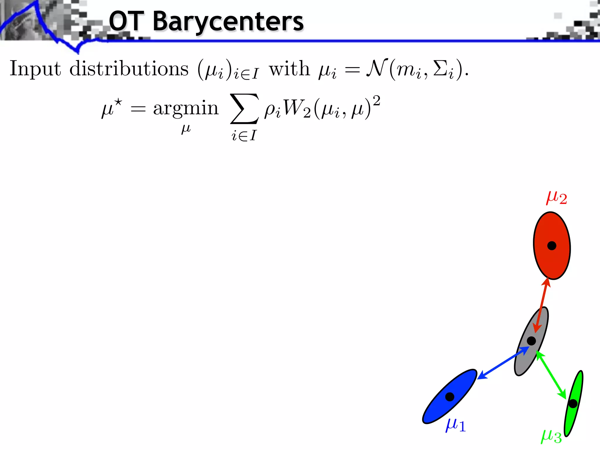
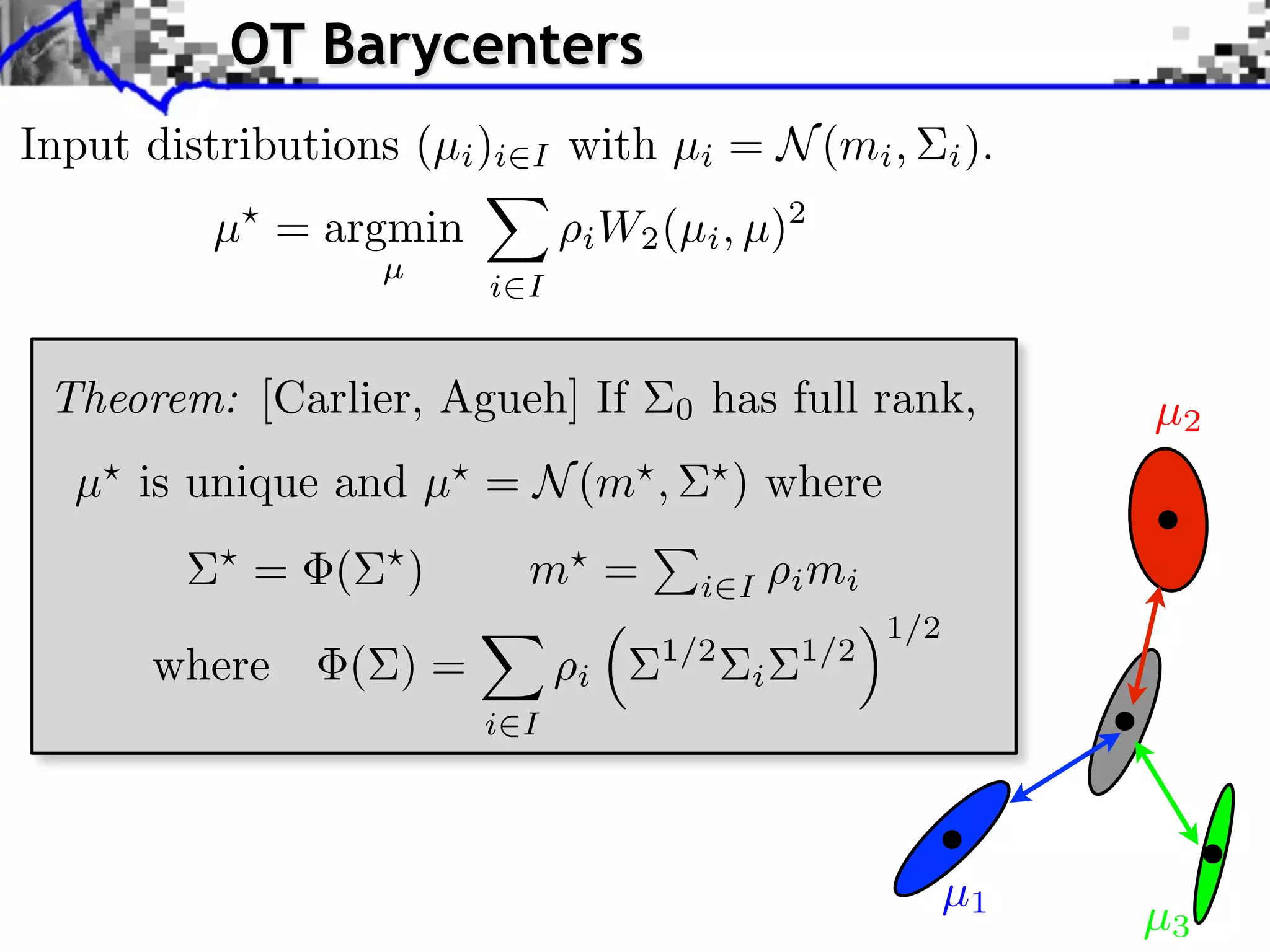
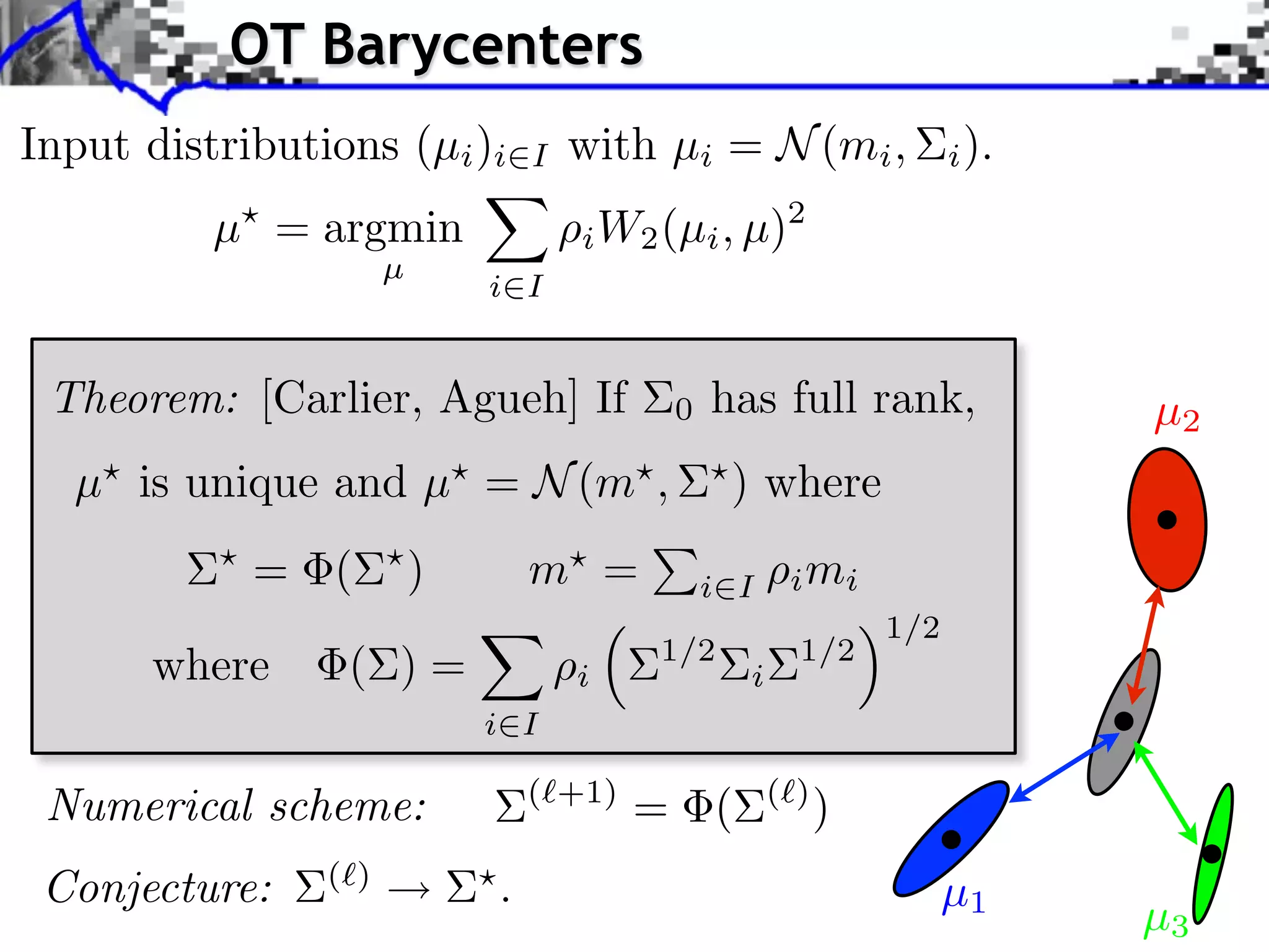
![Wasserstein Barycenter
µ2
Barycenter of {(µi , )}L :
i i=1 i =1
)
L i
2,µ
µ argmin W2 (µi , µ)2
2 (µ
i µ
W
µ
i=1 µ1
)
W2
(µ 1, µ
If µi = Xi , then µ = W2
(µ 3
X
,µ
X =
)
i Xi µ3
i
Generalizes Euclidean barycenter.
Theorem: [Agueh, Carlier, 2010]
if µ0 does not vanish on small sets,
µ exists and is unique.](https://image.slidesharecdn.com/2012-06-21-orsay-121213050319-phpapp01/75/Optimal-Transport-in-Imaging-Sciences-42-2048.jpg)

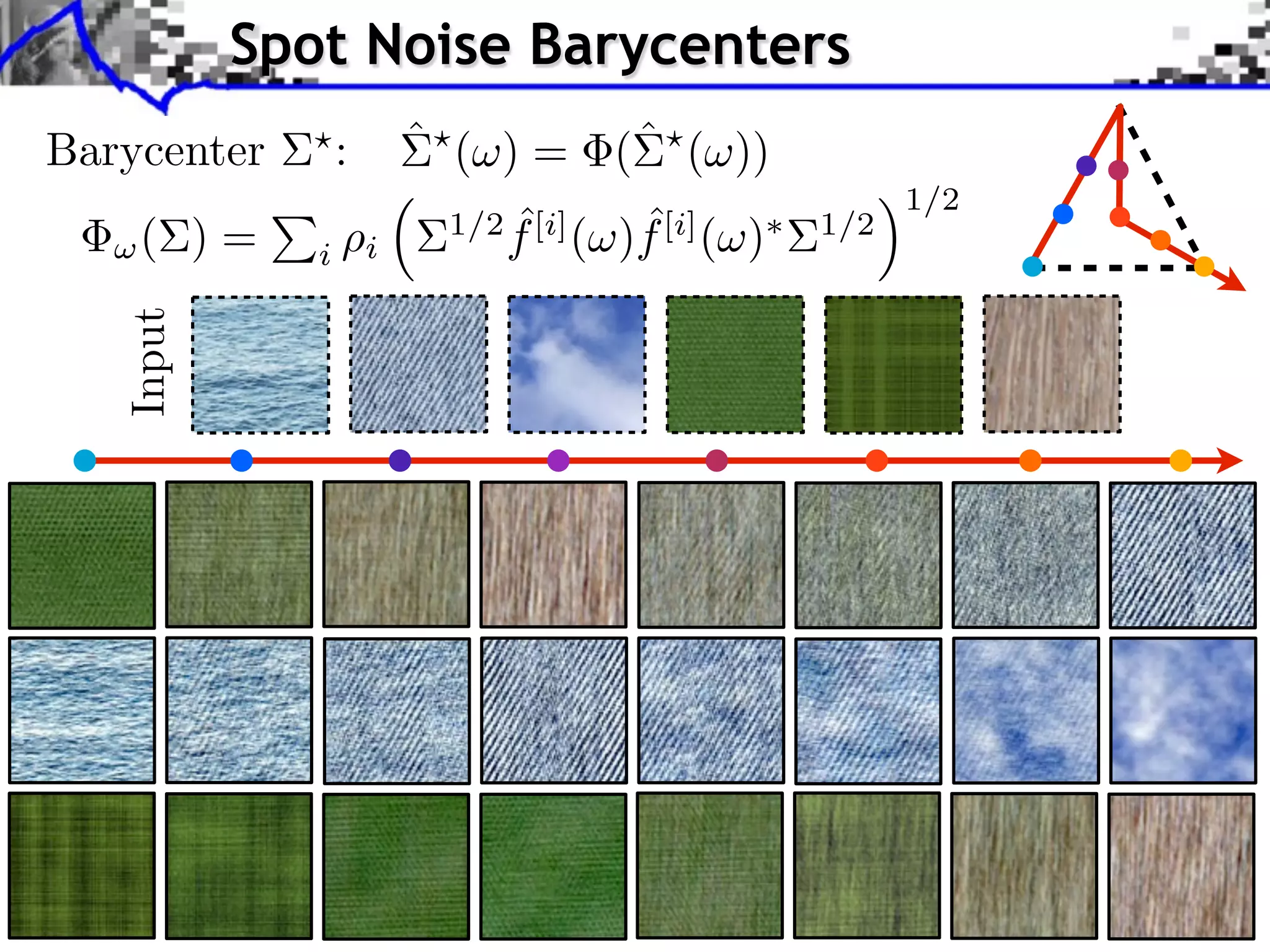
![Spot Noise Model [Galerne et al.]
Stationarity hypothesis: (periodic BC) X(· + ) X](https://image.slidesharecdn.com/2012-06-21-orsay-121213050319-phpapp01/75/Optimal-Transport-in-Imaging-Sciences-66-2048.jpg)
![Spot Noise Model [Galerne et al.]
Stationarity hypothesis: (periodic BC) X(· + ) X
Block-diagonal Fourier covariance:
ˆ
y = f computed as y ( ) = ˆ ( )f ( )
ˆ
2ix1 ⇥1 2ix2 ⇥2
ˆ
where f ( ) = f (x)e N1 + N2
x](https://image.slidesharecdn.com/2012-06-21-orsay-121213050319-phpapp01/75/Optimal-Transport-in-Imaging-Sciences-67-2048.jpg)
![Spot Noise Model [Galerne et al.]
Stationarity hypothesis: (periodic BC) X(· + ) X
Block-diagonal Fourier covariance:
ˆ
y = f computed as y ( ) = ˆ ( )f ( )
ˆ
2ix1 ⇥1 2ix2 ⇥2
ˆ
where f ( ) = f (x)e N1 + N2
x
Maximum likelihood estimate (MLE) of m from f0 :
1
i, mi = f0 (x) Rd
N x](https://image.slidesharecdn.com/2012-06-21-orsay-121213050319-phpapp01/75/Optimal-Transport-in-Imaging-Sciences-68-2048.jpg)
![Spot Noise Model [Galerne et al.]
Stationarity hypothesis: (periodic BC) X(· + ) X
Block-diagonal Fourier covariance:
ˆ
y = f computed as y ( ) = ˆ ( )f ( )
ˆ
2ix1 ⇥1 2ix2 ⇥2
ˆ
where f ( ) = f (x)e N1 + N2
x
Maximum likelihood estimate (MLE) of m from f0 :
1
i, mi = f0 (x) Rd
N x
1
MLE of : i,j = f0 (i + x) f0 (j + x) Rd d
N x](https://image.slidesharecdn.com/2012-06-21-orsay-121213050319-phpapp01/75/Optimal-Transport-in-Imaging-Sciences-69-2048.jpg)
![Spot Noise Model [Galerne et al.]
Stationarity hypothesis: (periodic BC) X(· + ) X
Block-diagonal Fourier covariance:
ˆ
y = f computed as y ( ) = ˆ ( )f ( )
ˆ
2ix1 ⇥1 2ix2 ⇥2
ˆ
where f ( ) = f (x)e N1 + N2
x
Maximum likelihood estimate (MLE) of m from f0 :
1
i, mi = f0 (x) Rd
N x
1
MLE of : i,j = f0 (i + x) f0 (j + x) Rd d
N x
ˆ ˆ
= 0, ˆ ( ) = f0 ( )f0 ( ) Cd d
is a spot noise = 0, ˆ ( ) is rank-1.](https://image.slidesharecdn.com/2012-06-21-orsay-121213050319-phpapp01/75/Optimal-Transport-in-Imaging-Sciences-70-2048.jpg)
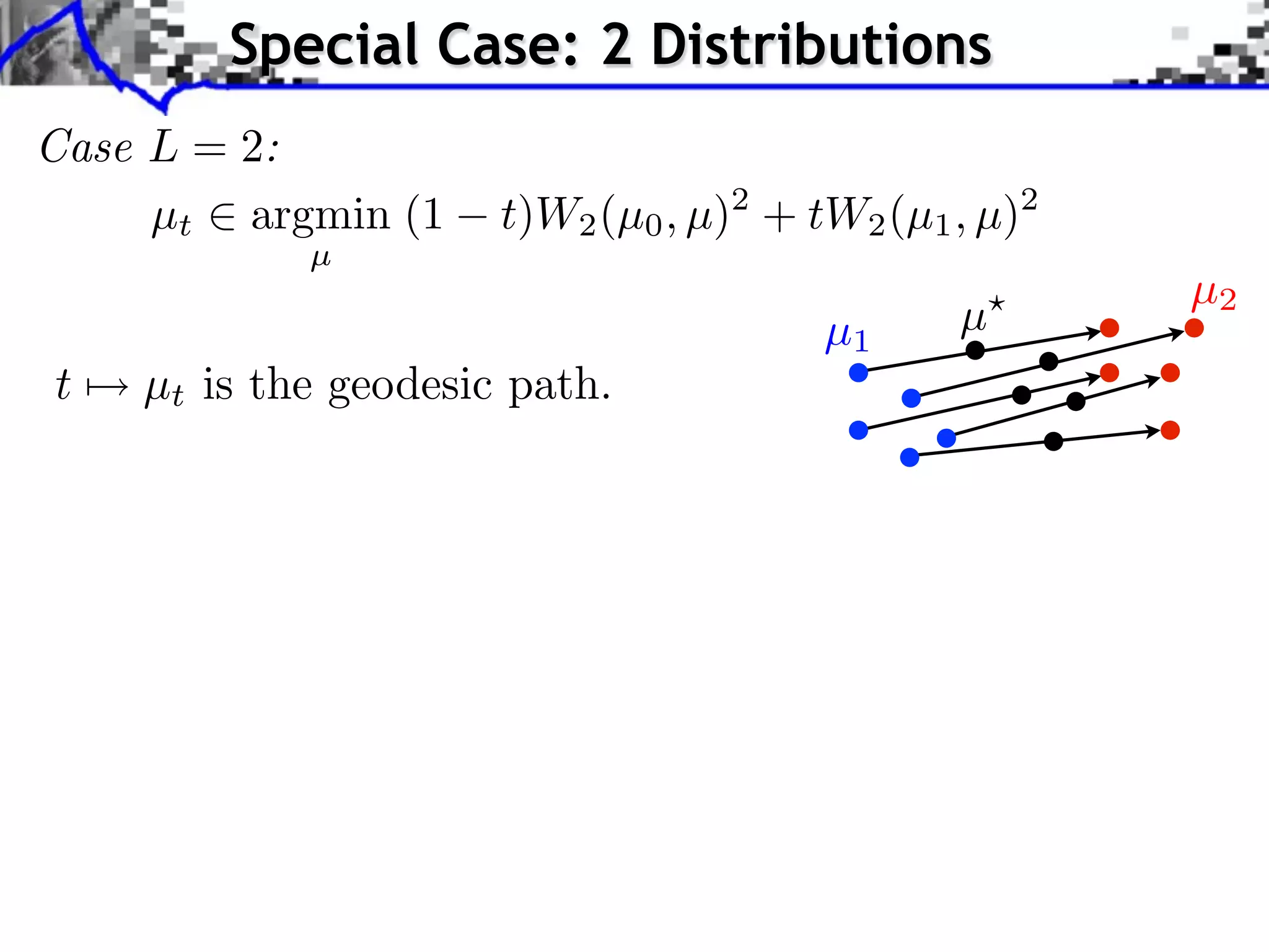
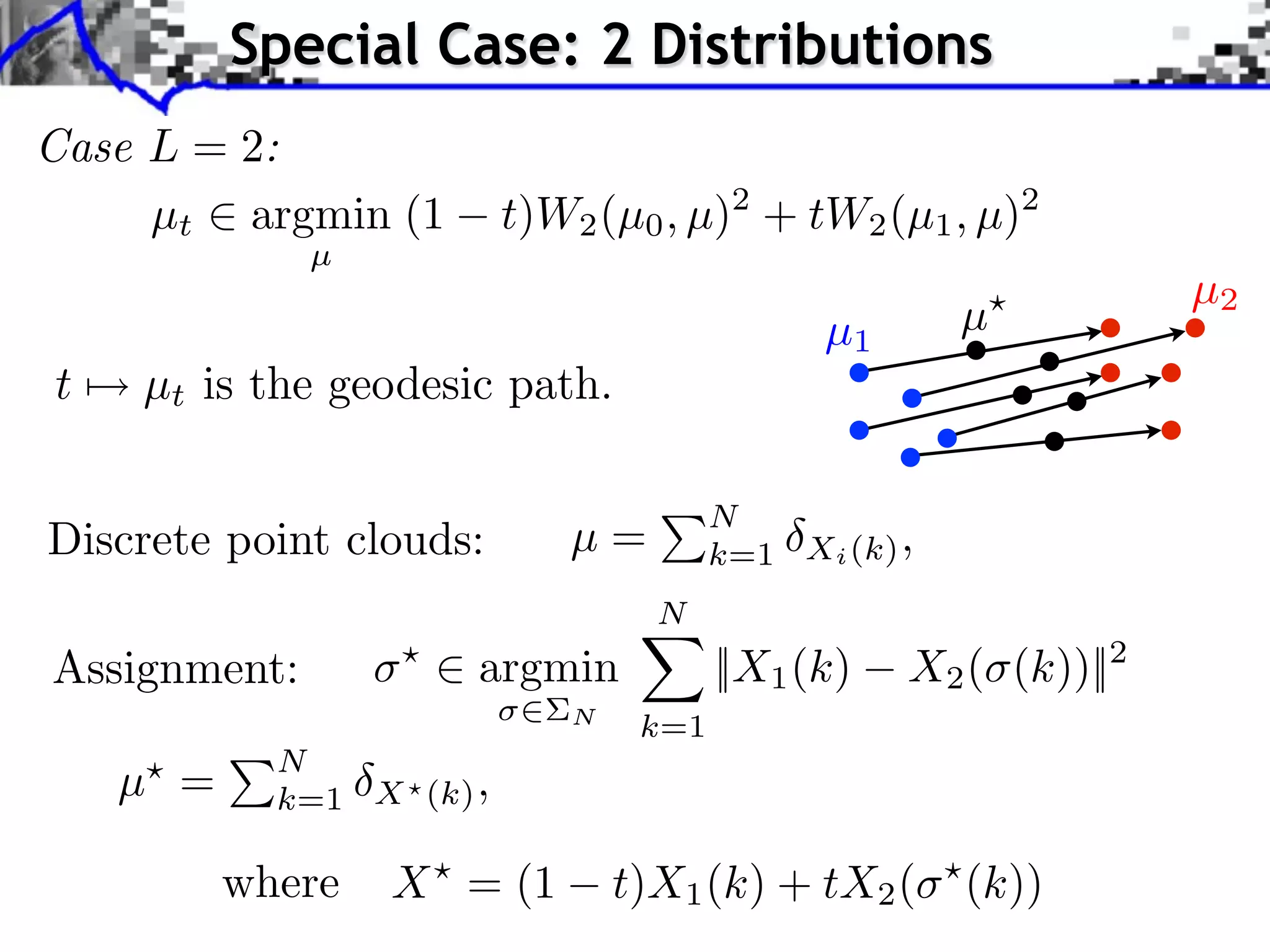
![Wasserstein Geodesics
Geodesics between (µ0 , µ1 ): t [0, 1] µt
Variational caracterization: (W2 is a geodesic distance)
µt = argmin (1 t)W2 (µ0 , µ)2 + tW2 (µ1 , µ)2
µ](https://image.slidesharecdn.com/2012-06-21-orsay-121213050319-phpapp01/75/Optimal-Transport-in-Imaging-Sciences-74-2048.jpg)
![Wasserstein Geodesics
Geodesics between (µ0 , µ1 ): t [0, 1] µt
Variational caracterization: (W2 is a geodesic distance)
µt = argmin (1 t)W2 (µ0 , µ)2 + tW2 (µ1 , µ)2
µ µ1
µ0 µ
Optimal transport caracterization:
µt = ((1 t)Id + tT ) µ0](https://image.slidesharecdn.com/2012-06-21-orsay-121213050319-phpapp01/75/Optimal-Transport-in-Imaging-Sciences-75-2048.jpg)
![Wasserstein Geodesics
Geodesics between (µ0 , µ1 ): t [0, 1] µt
Variational caracterization: (W2 is a geodesic distance)
µt = argmin (1 t)W2 (µ0 , µ)2 + tW2 (µ1 , µ)2
µ µ1
µ0 µ
Optimal transport caracterization:
µt = ((1 t)Id + tT ) µ0
µ0
Gaussian case: µt = Tt µ0 = N (mt , t)
mt = (1 t)m0 + tm1
t = [(1 t)Id + tT ] 0 [(1 t)Id + tT ]
the set of Gaussians is geodesically convex. µ1](https://image.slidesharecdn.com/2012-06-21-orsay-121213050319-phpapp01/75/Optimal-Transport-in-Imaging-Sciences-76-2048.jpg)
![Geodesic of Spot Noises
Theorem: Let for i = 0, 1, µi = µ(f [i] ) be spot noises,
ˆ ˆ
i.e. ˆ i ( ) = f [i] ( )f [i] ( ) . Then t [0, 1], µt = µ(f [t] )
f [t] = (1 t)f [0] + tg [1]
ˆ
f [1] ( ) ˆ
f [0] ( )
ˆ
g [1] ( ) = f [1] ( )
ˆ
ˆ
|f [1] ( ) ˆ
f [0] ( )|](https://image.slidesharecdn.com/2012-06-21-orsay-121213050319-phpapp01/75/Optimal-Transport-in-Imaging-Sciences-77-2048.jpg)
![Geodesic of Spot Noises
Theorem: Let for i = 0, 1, µi = µ(f [i] ) be spot noises,
ˆ ˆ
i.e. ˆ i ( ) = f [i] ( )f [i] ( ) . Then t [0, 1], µt = µ(f [t] )
f [t] = (1 t)f [0] + tg [1]
ˆ
f [1] ( ) ˆ
f [0] ( )
ˆ
g [1] ( ) = f [1] ( )
ˆ
ˆ
|f [1] ( ) ˆ
f [0] ( )|
f [0] t f [1]
0 1](https://image.slidesharecdn.com/2012-06-21-orsay-121213050319-phpapp01/75/Optimal-Transport-in-Imaging-Sciences-78-2048.jpg)

![Results following the geodesic path: 3
Abstract.- This paper tackles static and dynamic texture mixing by combining the statistical properties of an input set of images or videos. We focus on spot noise
images%%%%%%%%%%%%%%%%%%%%%%%%%%%%%%%%%%%%%%%%%%%%%%%%%%%%%%%%%%%%%%%%%%%%%%%%%%%%
Dynamic Textures Mixing
textures that follow a stationary and Gaussian model which can be learned from the given exemplars. From here, we define, using optimal transport, the distance
f [0] f [1] f [2]
between texture models, derive the geodesic path, and define the barycenter between several texture 2 models. These derivations are useful because they allow the
4
user to navigate inside the set of texture A T L A interpolating a new texture model at each element 1 the set. From these new interpolated models, new textures
M models, B C O D E of
5
can be synthesized of arbitrary size in space and time. Numerical results obtained from a library of exemplars show the ability of our method to generate new
complex realistic static and dynamic textures. 6
7
[See web page]
0
Results following the geodesic path: <%%%%%%%%%%%%%%%%%%%%%%%%%%%%%%%%%%%%%%%%%%%%%%%%%%%%%%%%%%%%%Start
3
images%%%%%%%%%%%%%%%%%%%%%%%%%%%%%%%%%%%%%%%%%%%%%%%%%%%%%%%%%%%%%
f [0] f [1]2 f [2]
MATLABCODE 4
1
0 1 5 2 3 4 5 6
6
Exemplars 0 7
<%%%%%%%%%%%%%%%%%%%%%%%%%%%%%%%%%%%%%%%%%%%%%%%%%%%%%%%%%%%%%Start
<%%%%%%%%%%%%%%%%%%%%%%%%%%%%%%%%%%%%%%%%%%%%%%%%%%%%%%%%%%%%%%%%
images%%%%%%%%%%%%%%%%%%%%%%%%%%%%%%%%%%%%%%%%%%%%%%%%%%%%%%%%%%%%%%%%%%%%%%%%%%%%
<%%%%%%%%%%%%%%%%%%%%%%%%%%%%%%%%%%%%%%%%%%%%%%%%%%%%%%%%%%%%%%%%
f [0] f [1] f [0] [2]
f [1] [2]
f f
0 1 2 3 4 5 6 7
<%%%%%%%%%%%%%%%%%%%%%%%%%%%%%%%%%%%%%%%%%%%%%%%%%%%%%%%%%%%%%%%%%%%%%%%%%%%%%%%
<%%%%%%%%%%%%%%%%%%%%%%%%%%%%%%%%%%%%%%%%%%%%%%%%%%%%%%%%%%%%%%%%%%%%%%%%>
f [0] [1] [2]
f 0 f 1 2 3 4 5 6
<%%%%%%%%%%%%%%%%%%%%%%%%%%%%%%%%%%%%%%%%%%%%%%%%%%%%%%%%%%%%%%%%
<%%%%%%%%%%%%%%%%%%%%%%%%%%%%%%%%%%%%%%%%%%%%%%%%%%%%%%%%%%%%%%%%
f [0] [1]
f
[2]
f
0 1 2 3 4 5 6
0 1 2 3 4 5 6 7
<%%%%%%%%%%%%%%%%%%%%%%%%%%%%%%%%%%%%%%%%%%%%%%%%%%%%%%%%%%%%%%%%
<%%%%%%%%%%%%%%%%%%%%%%%%%%%%%%%%%%%%%%%%%%%%%%%%%%%%%%%%%%%%%%%%%%%%%%%%%%%%%%%
<%%%%%%%%%%%%%%%%%%%%%%%%%%%%%%%%%%%%%%%%%%%%%%%%%%%%%%%%%%%%%%%%%%%%%%%%>
f [0] [1] [2]
f f
0 1 2 3 4 5 6 7](https://image.slidesharecdn.com/2012-06-21-orsay-121213050319-phpapp01/75/Optimal-Transport-in-Imaging-Sciences-85-2048.jpg)
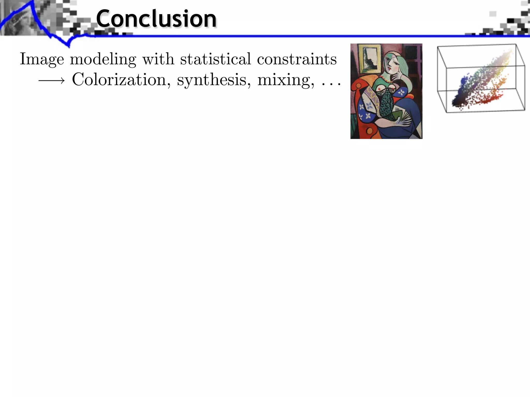
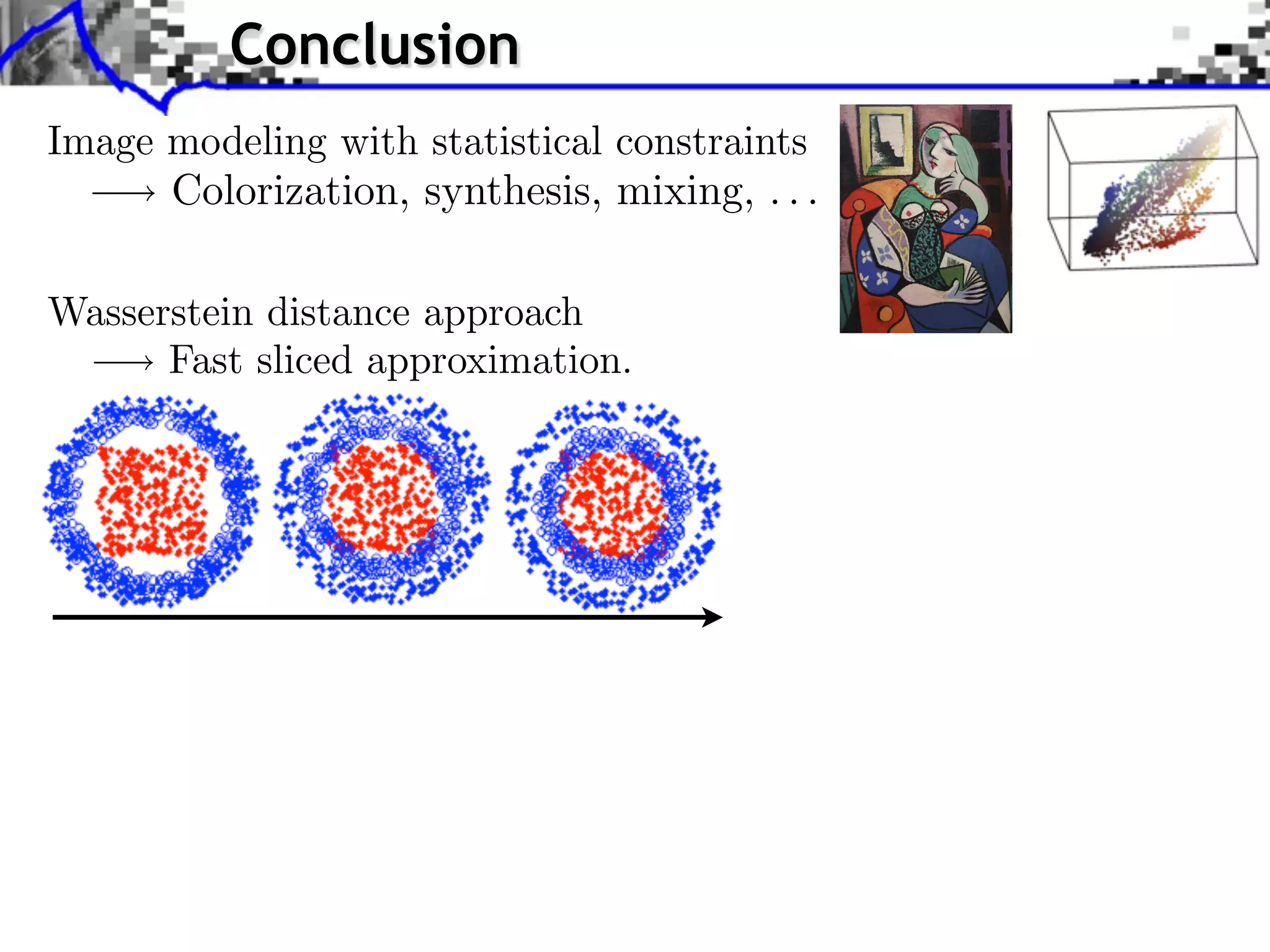
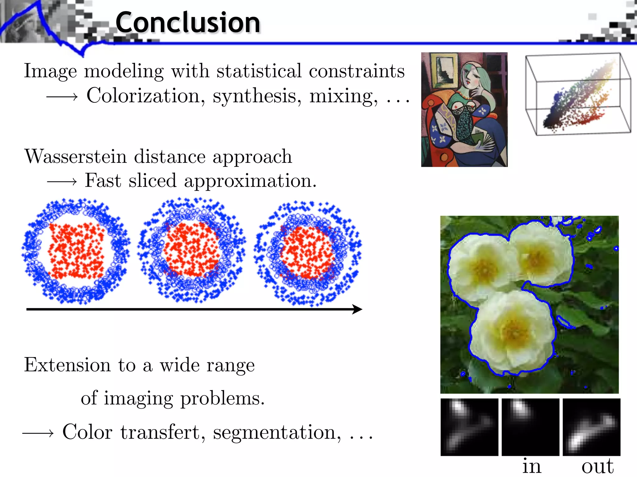

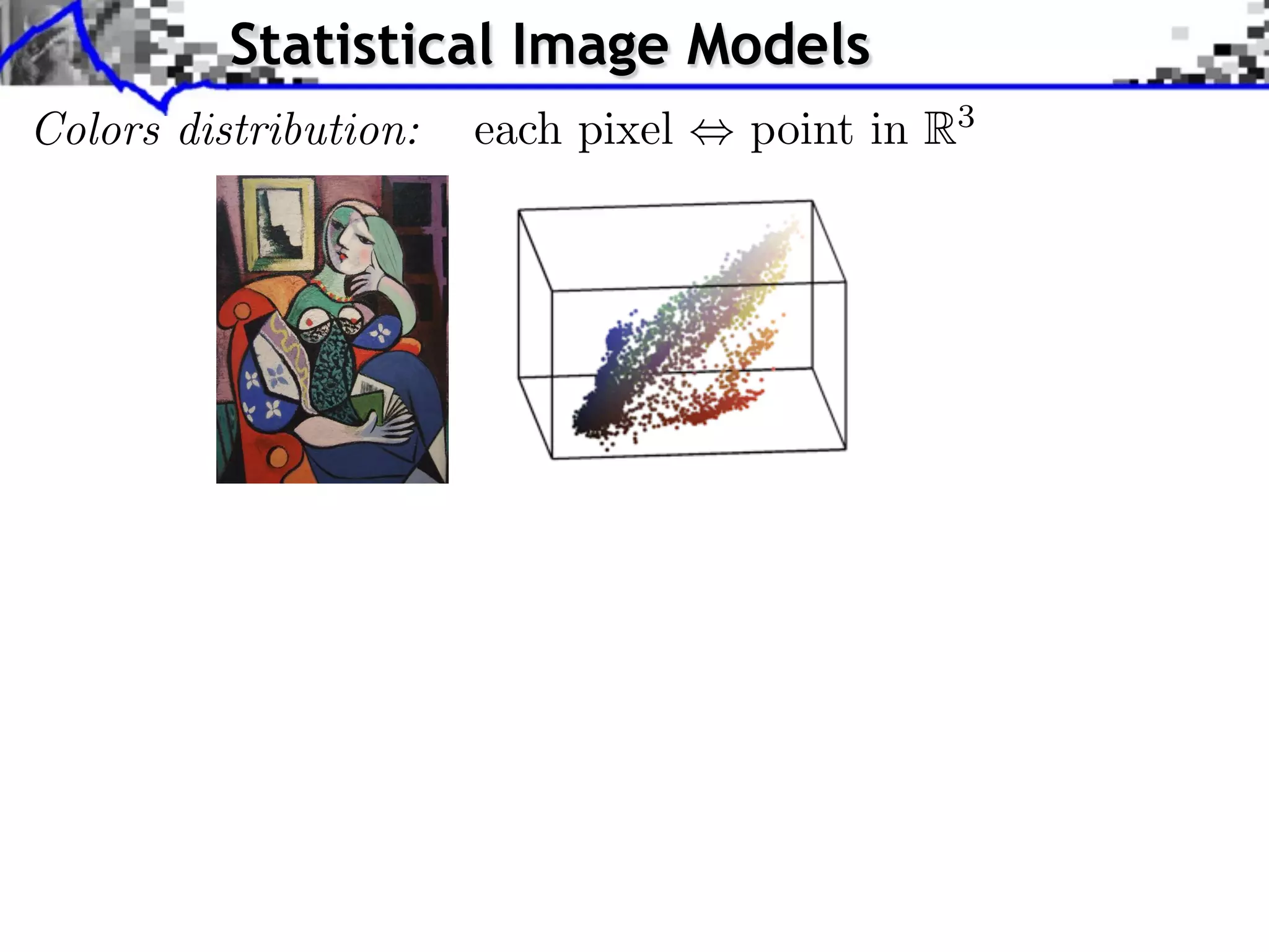
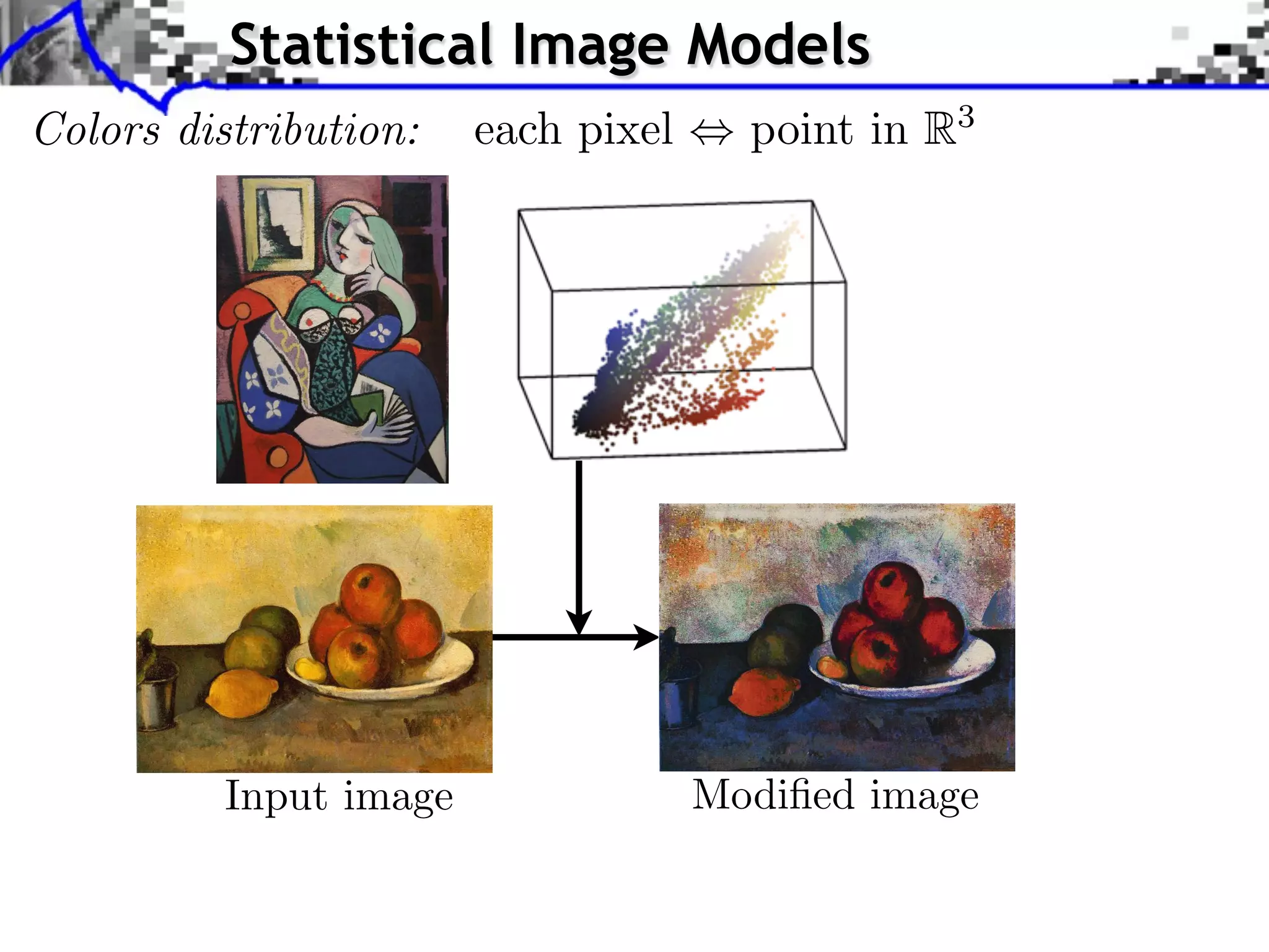
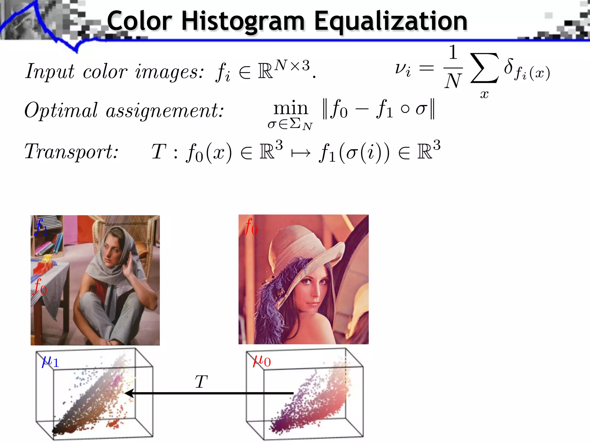
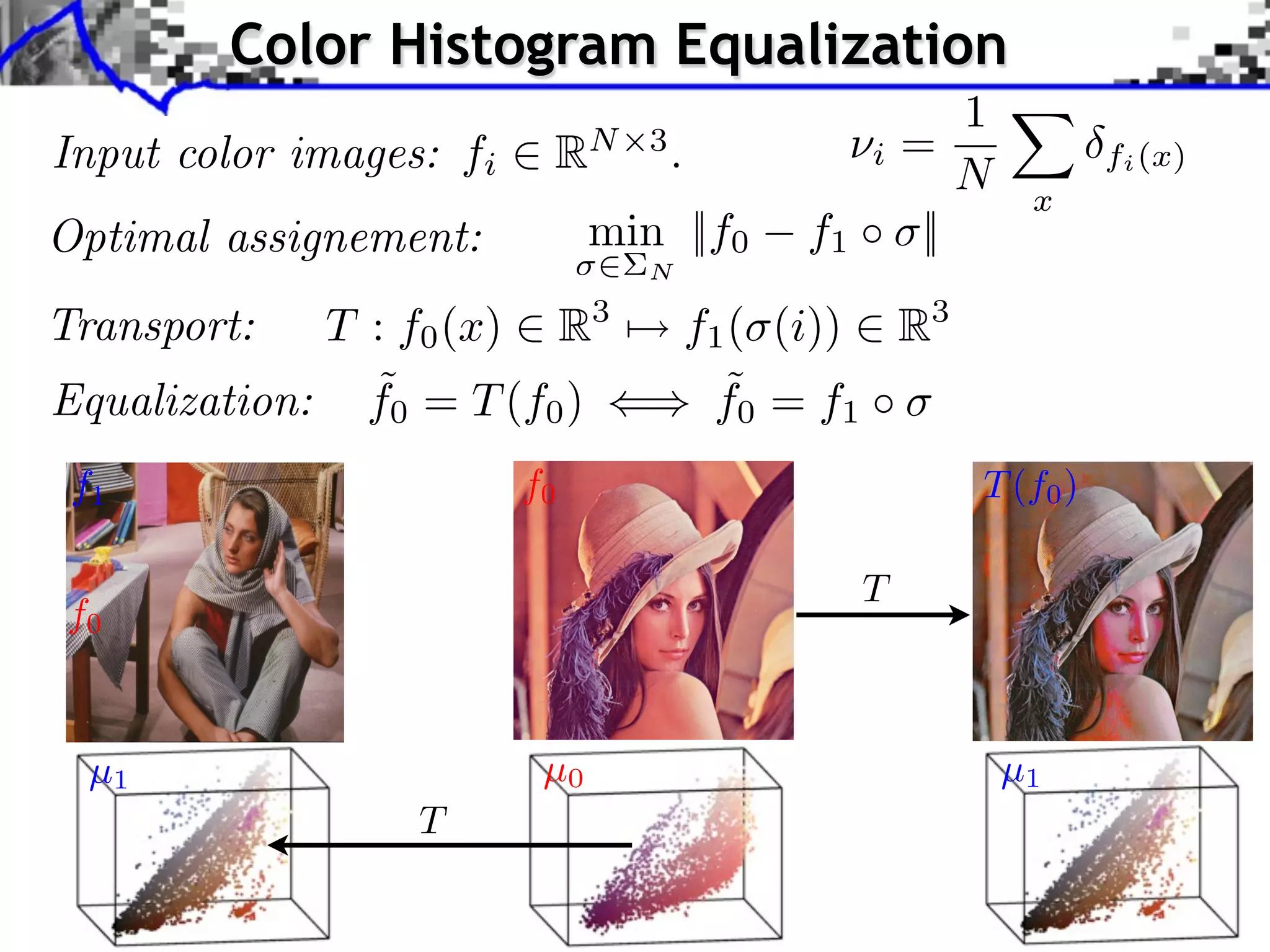
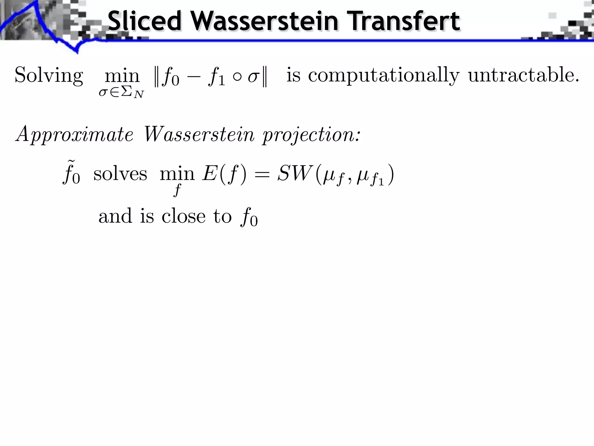
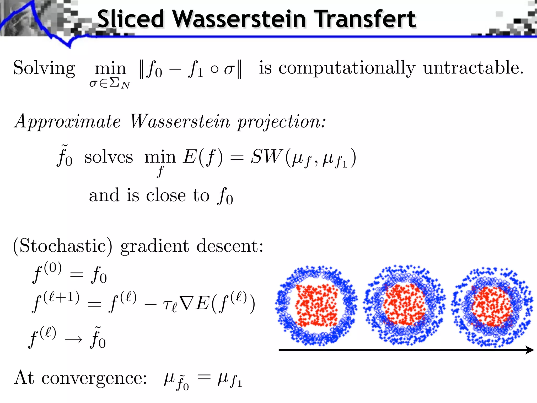
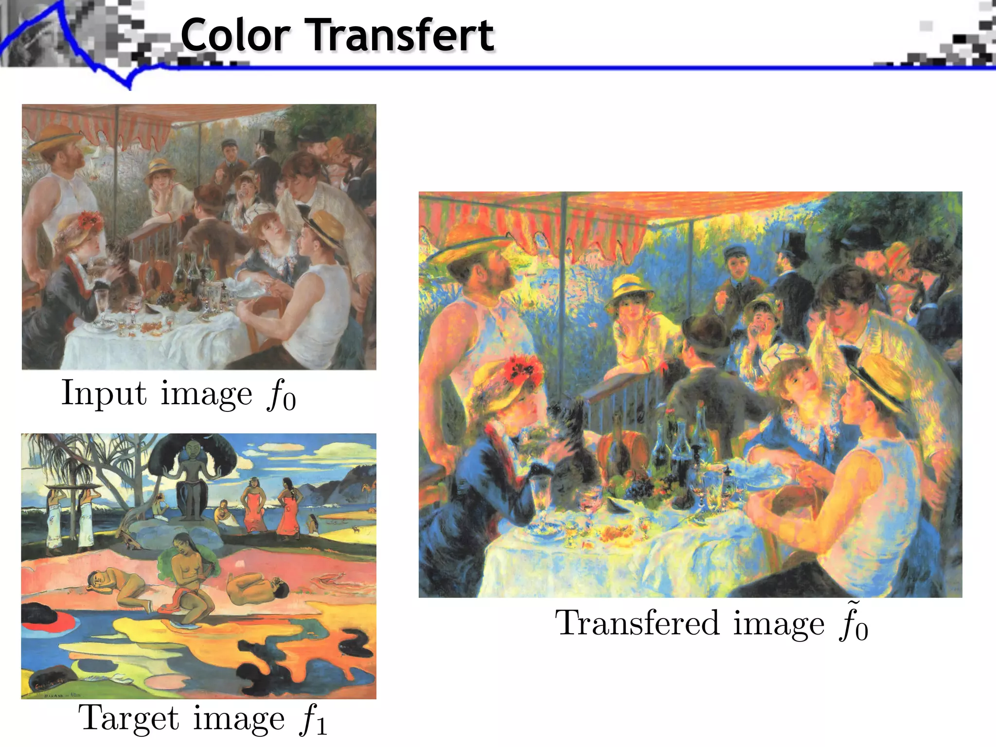
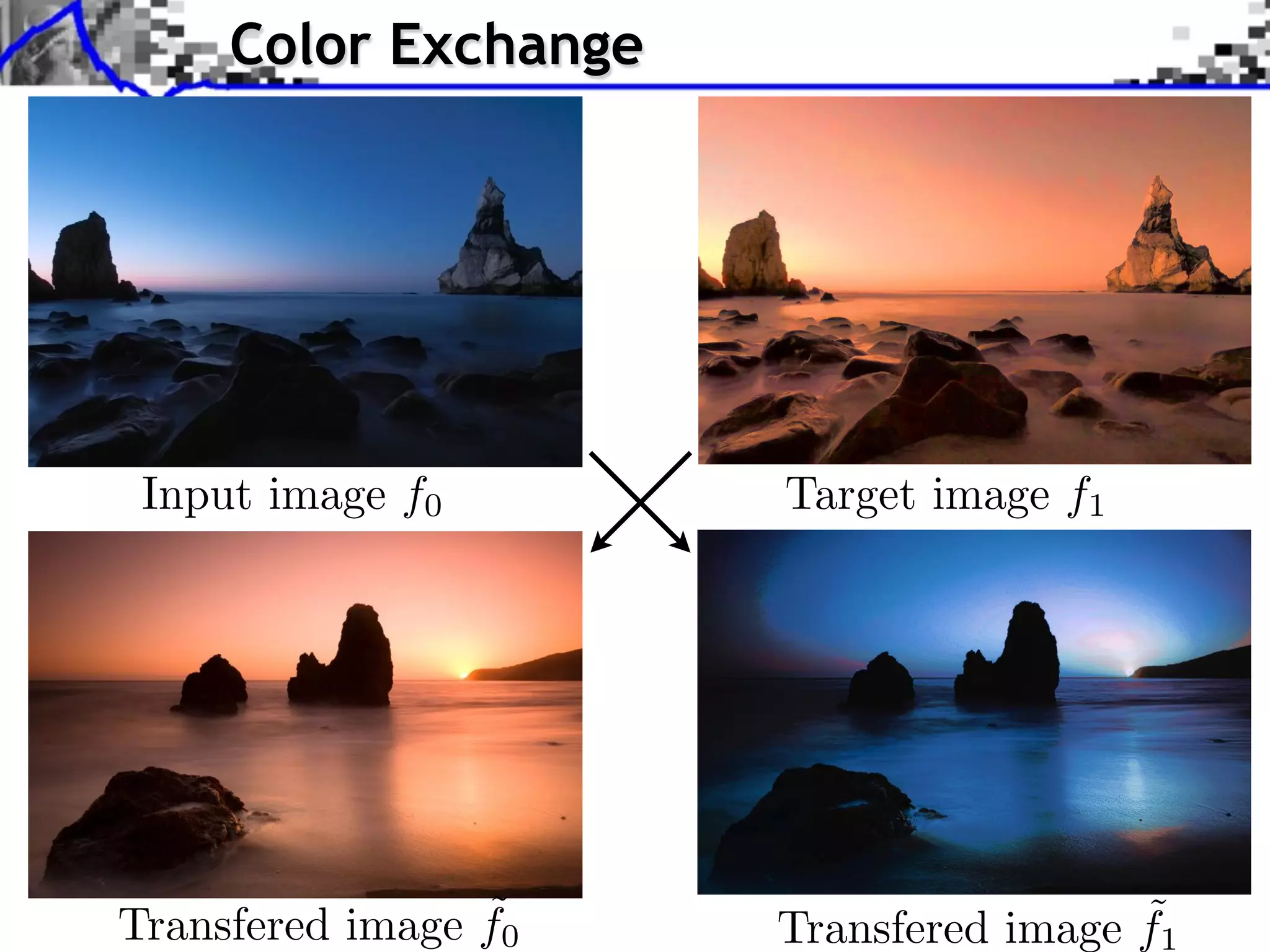
The document discusses optimal transport methods in imaging sciences, particularly focusing on the applications of the Wasserstein distance and sliced Wasserstein projections for color transfer and texture synthesis. It covers statistical image models, color statistics, and various numerical techniques for projecting images onto desired color distributions. Specific applications, challenges, and methods such as gradient descent and histogram equalization for color transfer are also highlighted.

![[第2回3D勉強会 研究紹介] Neural 3D Mesh Renderer (CVPR 2018)](https://cdn.slidesharecdn.com/ss_thumbnails/201807263dv-180728060959-thumbnail.jpg?width=640&height=640&fit=bounds)


![[DL輪読会]VNect: Real-time 3D Human Pose Estimation with a Single RGB Camera](https://cdn.slidesharecdn.com/ss_thumbnails/dl2018216vnect1-180323034835-thumbnail.jpg?width=640&height=640&fit=bounds)

![[DL輪読会]MetaFormer is Actually What You Need for Vision](https://cdn.slidesharecdn.com/ss_thumbnails/20220121metaformer-220121085750-thumbnail.jpg?width=640&height=640&fit=bounds)


![SSII2021 [SS1] Transformer x Computer Visionの 実活用可能性と展望 〜 TransformerのCompute...](https://cdn.slidesharecdn.com/ss_thumbnails/ss1-01-210607043349-thumbnail.jpg?width=640&height=640&fit=bounds)

![[DL輪読会]End-to-End Object Detection with Transformers](https://cdn.slidesharecdn.com/ss_thumbnails/200529dlseminardetr-200529061512-thumbnail.jpg?width=640&height=640&fit=bounds)
![[DL輪読会]A Bayesian Perspective on Generalization and Stochastic Gradient Descent](https://cdn.slidesharecdn.com/ss_thumbnails/20171106dl2-171108033614-thumbnail.jpg?width=640&height=640&fit=bounds)
![[DL輪読会]VoxelPose: Towards Multi-Camera 3D Human Pose Estimation in Wild Envir...](https://cdn.slidesharecdn.com/ss_thumbnails/20201023voxelposekuboshizuma-201023025841-thumbnail.jpg?width=640&height=640&fit=bounds)