Downloaded 1,110 times


![Patch-based Learning
Learning D
Exemplar patches yk Dictionary D
[Olshausen, Fields 1997]
State of the art denoising [Elad et al. 2006]](https://image.slidesharecdn.com/2012-05-15-ada7-121213110425-phpapp01/85/Learning-Sparse-Representation-37-320.jpg)
![Patch-based Learning
Learning D
Exemplar patches yk Dictionary D
[Olshausen, Fields 1997]
State of the art denoising [Elad et al. 2006]
Learning D
Sparse texture synthesis, inpainting [Peyr´ 2008]
e](https://image.slidesharecdn.com/2012-05-15-ada7-121213110425-phpapp01/85/Learning-Sparse-Representation-38-320.jpg)

![Patch-based Denoising
Noisy image: f = f0 + w.
Step 1: Extract patches. yk (·) = f (zk + ·)
yk
[Aharon & Elad 2006]](https://image.slidesharecdn.com/2012-05-15-ada7-121213110425-phpapp01/85/Learning-Sparse-Representation-41-320.jpg)
![Patch-based Denoising
Noisy image: f = f0 + w.
Step 1: Extract patches. yk (·) = f (zk + ·)
Step 2: Dictionary learning.
1
min ||yk Dxk || + ||xk ||1
2
D,(xk )k 2
k
yk
[Aharon & Elad 2006]](https://image.slidesharecdn.com/2012-05-15-ada7-121213110425-phpapp01/85/Learning-Sparse-Representation-42-320.jpg)
![Patch-based Denoising
Noisy image: f = f0 + w.
Step 1: Extract patches. yk (·) = f (zk + ·)
Step 2: Dictionary learning.
1
min ||yk Dxk || + ||xk ||1
2
D,(xk )k 2
k
Step 3: Patch averaging. yk = Dxk
˜
˜
f (·) ⇥ yk (· zk )
˜
k
yk ˜
yk
[Aharon & Elad 2006]](https://image.slidesharecdn.com/2012-05-15-ada7-121213110425-phpapp01/85/Learning-Sparse-Representation-43-320.jpg)


![Inpainting Example
LEARNING MULTISCALE AND SPARSE REPRESENTATIONS
LEARNING MULTISCALE AND SPARSE REPRESENTATIONS 237
237
(a) Original (b) Damaged
Image f0
(a) Original
(a) Original
Observations
(c) Restored, N = 1
(b) Damaged
(b) Damaged
Regularized f
(d) Restored, N = 2
y = using + w
Fig. 14. Inpainting f0 N = 2 and n = 16 × 16 (bottom-right image), or N = 1 and n = 8 × 8
(bottom-left). J = 100 iterations were performed, producing an adaptive dictionary. During the
learning, 50% of the patches were used. A sparsity factor L = 10 has been used during the learning
process and L = 25 for the final reconstruction. The damaged image was created by removing 75% of
the data from the original image. The initial PSNR is 6.13dB. The resulting PSNR for N = 2 is
[Mairal et al. 2008]
33.97dB and 31.75dB for N = 1.](https://image.slidesharecdn.com/2012-05-15-ada7-121213110425-phpapp01/85/Learning-Sparse-Representation-48-320.jpg)
![Adaptive Inpainting and Separation
Wavelets Local DCT
Wavelets Local DCT Learned
[Peyr´, Fadili, Starck 2010]
e](https://image.slidesharecdn.com/2012-05-15-ada7-121213110425-phpapp01/85/Learning-Sparse-Representation-49-320.jpg)

![OISING ALGORITHM WITH 256 ATOMS OF SIZE 7 7 3 FOR
TS ARE THOSE GIVEN BY MCAULEY AND AL [28] WITH THEIR “3
D DICTIONARY. THE BOTTOM-RIGHT ARE THE IMPROVEMENTS OBTAINED WITH THE ADAPTIVE APPRO
SENTATION FOR COLOR IMAGE RESTORATION
EST RESULTS FOR EACH GROUP. AS CAN BE SEEN, OUR PROPOSED TECHNIQUE CONSISTENTLY PRODUC
K-SVD ALGORITHM [2] ON EACH CHANNEL SEPARATELY WITH 8 8 ATOMS. THE BOTTOM-LEFT AR
s are reduced with our proposed technique (
Higher Dimensional Learning
mples of color artifacts while reconstructing a damaged version of the image (a) without the improvement here proposed ( in the new metric).
in our proposed new metric). Both images have been denoised with the same global dictionary.
bserves a bias effect in the color from the castle and in some part of the water. What is more, the color of the sky is piecewise constant when MAIRAL
rs), which is another artifact our approach corrected. (a) Original. (b) Original algorithm,
dB.
dB. (c) Proposed algorithm,
et al.: SPARSE REPRESENTATION FOR COLOR IMAGE RESTORATION
naries with 256 atoms learned on a generic database of natural images, with two different sizes of patches. Note the large number of color-less atoms.
can have negative values, the vectors are presented scaled and shifted to the [0,255] range per channel: (a) 5 5 3 patches; (b) 8 8 3 patches.
OLOR IMAGE RESTORATION 61
Fig. 7. Data set used for evaluating denoising experiments.
Learning D
(a) Training Image; (b) resulting dictionary; (b) is the dictionary learned in the image in (a). The dictionary is more colored than the global one.
TABLE I
Fig. 7. Data set used for evaluating denoising experiments.
les of color artifacts while reconstructing a damaged version of the image (a) without the improvement here proposedatoms learned on new metric).
Fig. 2. Dictionaries with 256 ( in the a generic database of natural images, with two d
are reduced with our proposed technique ( TABLE I our proposed new metric). Both images have been denoised negative values, the vectors are presented scaled and shifted to the [0,2
in
Since the atoms can have
with the same global dictionary.
ervesITH 256 ATOMS OF SIZE castle and in3 FOR of the water. What is more, the color of the sky is . EACH constant IS DIVIDED IN FOUR
W a bias effect in the color from the 7 7 some part AND 6 6 3 FOR piecewise CASE when
EN BY is another artifact our approach corrected. (a)HEIR “3(b) Original algorithm, HE TOP-RIGHT RESULTS ARE THOSE OBTAINED BY
), which
MCAULEY AND AL [28] WITH T Original. 3 MODEL.” T dB. (c) Proposed algorithm,
3 MODEL.” THE TOP-RIGHT RESUL
dB.
AND 6
M [2] ON EACH CHANNEL SEPARATELY WITH 8 8 ATOMS. THE BOTTOM-LEFT ARE OUR RESULTS OBTAINED
E BOTTOM-RIGHT ARE THE IMPROVEMENTS OBTAINED WITH THE ADAPTIVE APPROACH WITH 20 ITERATIONS.
EACH GROUP. AS CAN BE SEEN, OUR PROPOSED TECHNIQUE CONSISTENTLY PRODUCES THE BEST RESULTS
6 3 FOR . EAC](https://image.slidesharecdn.com/2012-05-15-ada7-121213110425-phpapp01/85/Learning-Sparse-Representation-51-320.jpg)
![OISING ALGORITHM WITH 256 ATOMS OF SIZE 7 7 3 FOR
TS ARE THOSE GIVEN BY MCAULEY AND AL [28] WITH THEIR “3
D DICTIONARY. THE BOTTOM-RIGHT ARE THE IMPROVEMENTS OBTAINED WITH THE ADAPTIVE APPRO
SENTATION FOR COLOR IMAGE RESTORATION
EST RESULTS FOR EACH GROUP. AS CAN BE SEEN, OUR PROPOSED TECHNIQUE CONSISTENTLY PRODUC
K-SVD ALGORITHM [2] ON EACH CHANNEL SEPARATELY WITH 8 8 ATOMS. THE BOTTOM-LEFT AR
Higher Dimensional Learning
O NLINE L EARNING FOR M ATRIX FACTORIZATION AND FACTORIZATION AND S PARSE C ODING
O NLINE L EARNING FOR M ATRIX S PARSE C ODING
mples of color artifacts while reconstructing a damaged version of the image (a) without the improvement here proposed (
s are reduced with our proposed technique (
in the new metric).
in our proposed new metric). Both images have been denoised with the same global dictionary.
bserves a bias effect in the color from the castle and in some part of the water. What is more, the color of the sky is piecewise constant when MAIRAL
rs), which is another artifact our approach corrected. (a) Original. (b) Original algorithm,
dB.
dB. (c) Proposed algorithm,
et al.: SPARSE REPRESENTATION FOR COLOR IMAGE RESTORATION
naries with 256 atoms learned on a generic database of natural images, with two different sizes of patches. Note the large number of color-less atoms.
can have negative values, the vectors are presented scaled and shifted to the [0,255] range per channel: (a) 5 5 3 patches; (b) 8 8 3 patches.
OLOR IMAGE RESTORATION 61
Fig. 7. Data set used for evaluating denoising experiments.
Learning D
(a) Training Image; (b) resulting dictionary; (b) is the dictionary learned in the image in (a). The dictionary is more colored than the global one.
TABLE I
Fig. 7. Data set used for evaluating denoising experiments.
les of color artifacts while reconstructing a damaged version of the image (a) without the improvement here proposedatoms learned on new metric).
Fig. 2. Dictionaries with 256 ( in the a generic database of natural images, with two d
are reduced with our proposed technique ( TABLE I our proposed new metric). Both images have been denoised negative values, the vectors are presented scaled and shifted to the [0,2
in
Since the atoms can have
with the same global dictionary.
ervesITH 256 ATOMS OF SIZE castle and in3 FOR of the water. What is more, the color of the sky is . EACH constant IS DIVIDED IN FOUR
W a bias effect in the color from the 7 7 some part AND 6 6 3 FOR piecewise CASE when
EN BY is another artifact our approach corrected. (a)HEIR “3(b) Original algorithm, HE TOP-RIGHT RESULTS ARE THOSE OBTAINED BY
), which
MCAULEY AND AL [28] WITH T Original. 3 MODEL.” T dB. (c) Proposed algorithm,
3 MODEL.” THE TOP-RIGHT RESUL
dB.
AND 6
M [2] ON EACH CHANNEL SEPARATELY WITH 8 8 ATOMS. THE BOTTOM-LEFT ARE OUR RESULTS OBTAINED
E BOTTOM-RIGHT ARE THE IMPROVEMENTS OBTAINED WITH THE ADAPTIVE APPROACH WITH 20 ITERATIONS. Inpainting
EACH GROUP. AS CAN BE SEEN, OUR PROPOSED TECHNIQUE CONSISTENTLY PRODUCES THE BEST RESULTS
6 3 FOR . EAC](https://image.slidesharecdn.com/2012-05-15-ada7-121213110425-phpapp01/85/Learning-Sparse-Representation-52-320.jpg)

![Facial Image Compression O. Bryt, M. Elad / J. Vis. Commun. Image R. 19 (2008) 270–282 271
[Elad et al. 2009]
show recognizable faces. We use a database containing around 6000
such facial images, some of which are used for training and tuning
the algorithm, and the others for testing it, similar to the approach
Image registration.
taken in [17].
In our work we propose a novel compression algorithm, related
to the one presented in [17], improving over it.
Our algorithm relies strongly on recent advancements made in
using sparse and redundant representation of signals [18–26], and
learning their sparsifying dictionaries [27–29]. We use the K-SVD
algorithm for learning the dictionaries for representing small
image patches in a locally adaptive way, and use these to sparse-
code the patches’ content. This is a relatively simple and
straight-forward algorithm with hardly any entropy coding stage.
Yet, it is shown to be superior to several competing algorithms:
(i) the JPEG2000, (ii) the VQ-based algorithm presented in [17],
and (iii) A Principal Component Analysis (PCA) approach.2 Fig. 1. (Left) Piece-wise affine warping of the image by triangulation. (Right) A
In the next section we provide some background material for uniform slicing to disjoint square patches for coding purposes.
this work: we start by presenting the details of the compression
algorithm developed in [17], as their scheme is the one we embark K-Means) per each patch separately, using patches taken from the
from in the development of ours. We also describe the topic of same location from 5000 training images. This way, each VQ is
sparse and redundant representations and the K-SVD, that are adapted to the expected local content, and thus the high perfor-
the foundations for our algorithm. In Section 3 we turn to present mance presented by this algorithm. The number of code-words
the proposed algorithm in details, showing its various steps, and in the VQ is a function of the bit-allocation for the patches. As
discussing its computational/memory complexities. Section 4 we argue in the next section, VQ coding is limited by the available
presents results of our method, demonstrating the claimed number of examples and the desired rate, forcing relatively small
superiority. We conclude in Section 5 with a list of future activities patch sizes. This, in turn, leads to a loss of some redundancy be-
that can further improve over the proposed scheme. tween adjacent patches, and thus loss of potential compression.
Another ingredient in this algorithm that partly compensates
2. Background material for the above-described shortcoming is a multi-scale coding
scheme. The image is scaled down and VQ-coded using patches
2.1. VQ-based image compression of size 8 Â 8. Then it is interpolated back to the original resolution,
and the residual is coded using VQ on 8 Â 8 pixel patches once
Among the thousands of papers that study still image again. This method can be applied on a Laplacian pyramid of the
compression algorithms, there are relatively few that consider original (warped) image with several scales [33].
the treatment of facial images [2–17]. Among those, the most As already mentioned above, the results shown in [17] surpass
recent and the best performing algorithm is the one reported in those obtained by JPEG2000, both visually and in Peak-Signal-to-
[17]. That paper also provides a thorough literature survey that Noise Ratio (PSNR) quantitative comparisons. In our work we pro-
compares the various methods and discusses similarities and pose to replace the coding stage from VQ to sparse and redundant
differences between them. Therefore, rather than repeating such representations—this leads us to the next subsection, were we de-
a survey here, we refer the interested reader to [17]. In this scribe the principles behind this coding strategy.
sub-section we concentrate on the description of the algorithm
in [17] as our method resembles it to some extent. 2.2. Sparse and redundant representations](https://image.slidesharecdn.com/2012-05-15-ada7-121213110425-phpapp01/85/Learning-Sparse-Representation-54-320.jpg)
![Facial Image Compression O.O. Bryt, M. EladJ. J. Vis. Commun. Image R. 19 (2008) 270–282
Bryt, M. Elad / / Vis. Commun. Image R. 19 (2008) 270–282 271
271
[Elad et al. 2009]
show recognizable faces. We use a a database containing around 6000
show recognizable faces. We use database containing around 6000
such facial images, some of which are used for training and tuning
such facial images, some of which are used for training and tuning
the algorithm, and the others for testing it, similar to the approach
the algorithm, and the others for testing it, similar to the approach
Image registration.
taken in [17].
taken in [17].
In our work we propose a a novel compression algorithm, related
In our work we propose novel compression algorithm, related
to the one presented in [17], improving over it.
to the one presented in [17], improving over it.
Our algorithm relies strongly on recent advancements made in
Our algorithm relies strongly on recent advancements made in
Non-overlapping patches (fk )k .
using sparse and redundant representation of signals [18–26], and
using sparse and redundant representation of signals [18–26], and fk
learning their sparsifying dictionaries [27–29]. We use the K-SVD
learning their sparsifying dictionaries [27–29]. We use the K-SVD
algorithm for learning the dictionaries for representing small
algorithm for learning the dictionaries for representing small
image patches in a a locally adaptive way, and use these to sparse-
image patches in locally adaptive way, and use these to sparse-
code the patches’ content. This isis a a relatively simple and
code the patches’ content. This relatively simple and
straight-forward algorithm with hardly any entropy coding stage.
straight-forward algorithm with hardly any entropy coding stage.
Yet, itit is shown to be superior to several competing algorithms:
Yet, is shown to be superior to several competing algorithms:
(i) the JPEG2000, (ii) the VQ-based algorithm presented in [17],
(i) the JPEG2000, (ii) the VQ-based algorithm presented in [17],
2
and (iii) AA Principal Component Analysis (PCA) approach.2
and (iii) Principal Component Analysis (PCA) approach. Fig. 1.1. (Left) Piece-wise affine warping of the image by triangulation. (Right) A
Fig. (Left) Piece-wise affine warping of the image by triangulation. (Right) A
In the next section we provide some background material for
In the next section we provide some background material for uniform slicing toto disjoint square patches for coding purposes.
uniform slicing disjoint square patches for coding purposes.
this work: we start by presenting the details of the compression
this work: we start by presenting the details of the compression
algorithm developed in [17], as their scheme isis the one we embark
algorithm developed in [17], as their scheme the one we embark K-Means) per each patch separately, using patches taken from the
K-Means) per each patch separately, using patches taken from the
from in the development of ours. We also describe the topic of
from in the development of ours. We also describe the topic of same location from 5000 training images. This way, each VQ isis
same location from 5000 training images. This way, each VQ
sparse and redundant representations and the K-SVD, that are
sparse and redundant representations and the K-SVD, that are adapted to the expected local content, and thus the high perfor-
adapted to the expected local content, and thus the high perfor-
the foundations for our algorithm. In Section 3 3 we turn to present
the foundations for our algorithm. In Section we turn to present mance presented by this algorithm. The number of code-words
mance presented by this algorithm. The number of code-words
the proposed algorithm in details, showing its various steps, and
the proposed algorithm in details, showing its various steps, and in the VQ isisa afunction of the bit-allocation for the patches. As
in the VQ function of the bit-allocation for the patches. As
discussing its computational/memory complexities. Section 4 4
discussing its computational/memory complexities. Section we argue in the next section, VQ coding isis limited by the available
we argue in the next section, VQ coding limited by the available
presents results of our method, demonstrating the claimed
presents results of our method, demonstrating the claimed number of examples and the desired rate, forcing relatively small
number of examples and the desired rate, forcing relatively small
superiority. We conclude in Section 5 5 with a list of future activities
superiority. We conclude in Section with a list of future activities patch sizes. This, in turn, leads to a a loss of some redundancy be-
patch sizes. This, in turn, leads to loss of some redundancy be-
that can further improve over the proposed scheme.
that can further improve over the proposed scheme. tween adjacent patches, and thus loss of potential compression.
tween adjacent patches, and thus loss of potential compression.
Another ingredient in this algorithm that partly compensates
Another ingredient in this algorithm that partly compensates
2. Background material
2. Background material for the above-described shortcoming isis a a multi-scale coding
for the above-described shortcoming multi-scale coding
scheme. The image isisscaled down and VQ-coded using patches
scheme. The image scaled down and VQ-coded using patches
2.1. VQ-based image compression
2.1. VQ-based image compression of size 8 8 Â 8. Then it is interpolated back to the original resolution,
of size  8. Then it is interpolated back to the original resolution,
and the residual isiscoded using VQ on 8 8 Â 8pixel patches once
and the residual coded using VQ on  8 pixel patches once
Among the thousands of papers that study still image
Among the thousands of papers that study still image again. This method can be applied on a a Laplacian pyramid of the
again. This method can be applied on Laplacian pyramid of the
compression algorithms, there are relatively few that consider
compression algorithms, there are relatively few that consider original (warped) image with several scales [33].
original (warped) image with several scales [33].
the treatment of facial images [2–17]. Among those, the most
the treatment of facial images [2–17]. Among those, the most As already mentioned above, the results shown in [17] surpass
As already mentioned above, the results shown in [17] surpass
recent and the best performing algorithm isis the one reported in
recent and the best performing algorithm the one reported in those obtained by JPEG2000, both visually and in Peak-Signal-to-
those obtained by JPEG2000, both visually and in Peak-Signal-to-
[17]. That paper also provides a athorough literature survey that
[17]. That paper also provides thorough literature survey that Noise Ratio (PSNR) quantitative comparisons. In our work we pro-
Noise Ratio (PSNR) quantitative comparisons. In our work we pro-
compares the various methods and discusses similarities and
compares the various methods and discusses similarities and pose to replace the coding stage from VQ to sparse and redundant
pose to replace the coding stage from VQ to sparse and redundant
differences between them. Therefore, rather than repeating such
differences between them. Therefore, rather than repeating such representations—this leads us to the next subsection, were we de-
representations—this leads us to the next subsection, were we de-
a asurvey here, we refer the interested reader to [17]. In this
survey here, we refer the interested reader to [17]. In this scribe the principles behind this coding strategy.
scribe the principles behind this coding strategy.
sub-section we concentrate on the description of the algorithm
sub-section we concentrate on the description of the algorithm
in [17] as our method resembles itit to some extent.
in [17] as our method resembles to some extent. 2.2. Sparse and redundant representations
2.2. Sparse and redundant representations](https://image.slidesharecdn.com/2012-05-15-ada7-121213110425-phpapp01/85/Learning-Sparse-Representation-55-320.jpg)
![Facial Image Compression O. Bryt, M. Elad / J. Vis. Commun. Image R. 19 (2008) 270–282
Before turning to preset the results we should add the follow-
O.O. Bryt, M. EladJ. J. ing: while all theImage R. 19 (2008) 270–282 specific database
Bryt, M. Elad / / Vis. Commun. Image R. shown here 270–282
Vis. Commun. results 19 (2008) refer to the
was trained for patch number 80 (The left
271
coding atoms, and similarly, in Fig. 7 we271
can
we operate on, the overall scheme proposed is general and should was trained for patch number 87 (The right
apply to other face images databases just as well. Naturally, some sparse coding atoms. It can be seen that bot
[Elad et al. 2009]
show recognizable faces. We use a a database containing around 6000 the parameters might be necessary, and among those,
show recognizable faces. We use database containing around 6000 in
changes images similar in nature to the image patch
such facial images, some of which are used for training and tuning size is the most important to consider. We also note that
such facial images, some of which are used for training andthe patch
tuning trained for. A similar behavior was observed
the algorithm, and the others for testing it, similar to the approach from one source of images to another, this relative size
as one shifts
the algorithm, and the others for testing it, similar to the approach
of the background in the photos may vary, and
the
necessarily 4.2. Reconstructed images
Image registration.
taken in [17].
taken in [17]. leads to changes in performance. More specifically, when the back-
In our work we propose a a novel compression algorithm, ground small such larger (e.g., the images we useperformance is
In our work we propose novel compression algorithm, related related
tively
regions are
regions),
the
compression
here have rela- Our coding strategy allows us to learn w
age are more difficult than others to co
to the one presented in [17], improving over it.
to the one presented in [17], improving over it. expected to improve. assigning the same representation error th
Our algorithm relies strongly on recent advancements made in
Our algorithm relies strongly on recent advancements made in dictionaries
Non-overlapping patches (fk )k .
4.1. K-SVD
using sparse and redundant representation of signals [18–26], and
using sparse and redundant representation of signals [18–26], and fk
patches, and observing how many atoms
representation of each patch on average.
a small number of allocated atoms are simp
learning their sparsifying dictionaries [27–29]. We use the K-SVD
learning their sparsifying dictionaries [27–29]. We use the K-SVDThe primary stopping condition for the training process was set others. We would expect that the represent
to be a limitation on the maximal number of K-SVD iterations of the image such as the background, p
algorithm for learning the dictionaries for representing (being 100). A secondary stopping condition was a limitation on
algorithm for learning the dictionaries for representingsmall small maybe parts of the clothes will be simpler
image patches in a a locally adaptive way, and use these to sparse-
image patches in locally adaptive way, and use these to sparse-
the minimal representation error. In the image compression stage tion of areas containing high frequency e
Dictionary learning (Dk )k .
we added a limitation on the maximal number of atoms per patch. hair or the eyes. Fig. 8 shows maps of atom
code the patches’ content. This isis a a relatively simple and
code the patches’ content. This relatively simple and
These conditions were used to allow us to better control the rates and representation error (RMSE—squared
straight-forward algorithm with hardly any entropy coding of stage.
stage.
straight-forward algorithm with hardly any entropy coding the resulting images and the overall simulation time. squared error) per patch for the images in
Every obtained dictionary contains 512 patches of size different bit-rates. It can be seen that more
Yet, itit is shown to be superior to several competing algorithms: as atoms. In Fig. 6 we can see the dictionary that
Yet, is shown to be superior to several competing algorithms:pixels
15 Â 15 to patches containing the facial details (h
(i) the JPEG2000, (ii) the VQ-based algorithm presented in [17],
(i) the JPEG2000, (ii) the VQ-based algorithm presented in [17],
2
and (iii) AA Principal Component Analysis (PCA) approach.2
and (iii) Principal Component Analysis (PCA) approach. Fig. 1.1. (Left) Piece-wise affine warping of the image by triangulation. (Right) A
Fig. (Left) Piece-wise affine warping of the image by triangulation. (Right) A
In the next section we provide some background material for
In the next section we provide some background material for uniform slicing toto disjoint square patches for coding purposes.
uniform slicing disjoint square patches for coding purposes.
this work: we start by presenting the details of the compression
this work: we start by presenting the details of the compression
algorithm developed in [17], as their scheme isis the one we embark
algorithm developed in [17], as their scheme the one we embark K-Means) per each patch separately, using patches taken from the
K-Means) per each patch separately, using patches taken from the
from in the development of ours. We also describe the topic of
from in the development of ours. We also describe the topic of same location from 5000 training images. This way, each VQ isis
same location from 5000 training images. This way, each VQ
sparse and redundant representations and the K-SVD, that are
sparse and redundant representations and the K-SVD, that are adapted to the expected local content, and thus the high perfor-
adapted to the expected local content, and thus the high perfor-
the foundations for our algorithm. In Section 3 3 we turn to present
the foundations for our algorithm. In Section we turn to present mance presented by this algorithm. The number of code-words
mance presented by this algorithm. The number of code-words
the proposed algorithm in details, showing its various steps, and
the proposed algorithm in details, showing its various steps, and in the VQ isisa afunction of the bit-allocation for the patches. As
in the VQ function of the bit-allocation for the patches. As
discussing its computational/memory complexities. Section 4 4
discussing its computational/memory complexities. Section we argue in the next section, VQ coding isis limited by the available
we argue in the next section, VQ coding limited by the available
presents results of our method, demonstrating the claimed
presents results of our method, demonstrating the claimed number of examples and the desired rate, forcing relatively small
number of examples and the desired rate, forcing relatively small
superiority. We conclude in Section 5 5 with a list of future activities
superiority. We conclude in Section with a list of future activities patch sizes. This, in turn, leads to a a loss of some redundancy be-
patch sizes. This, in turn, leads to loss of some redundancy be-
that can further improve over the proposed scheme.
that can further improve over the proposed scheme. tween adjacent patches, and thus loss of potential compression.
tween adjacent patches, and thus loss of potential compression.
2. Background material
2. Background material
AnotherThe Dictionary obtained by K-SVD for Patch No. 80 (the that partlyOMPcompensates
Another ingredient in this algorithmleft eye) using the compensates
Fig. 6. ingredient in this algorithm that partly method with L ¼ 4.
for the above-described shortcoming isis a a multi-scale coding
for the above-described shortcoming multi-scale coding
Dk
scheme. The image isisscaled down and VQ-coded using patches
scheme. The image scaled down and VQ-coded using patches
2.1. VQ-based image compression
2.1. VQ-based image compression of size 8 8 Â 8. Then it is interpolated back to the original resolution,
of size  8. Then it is interpolated back to the original resolution,
and the residual isiscoded using VQ on 8 8 Â 8pixel patches once
and the residual coded using VQ on  8 pixel patches once
Among the thousands of papers that study still image
Among the thousands of papers that study still image again. This method can be applied on a a Laplacian pyramid of the
again. This method can be applied on Laplacian pyramid of the
compression algorithms, there are relatively few that consider
compression algorithms, there are relatively few that consider original (warped) image with several scales [33].
original (warped) image with several scales [33].
the treatment of facial images [2–17]. Among those, the most
the treatment of facial images [2–17]. Among those, the most As already mentioned above, the results shown in [17] surpass
As already mentioned above, the results shown in [17] surpass
recent and the best performing algorithm isis the one reported in
recent and the best performing algorithm the one reported in those obtained by JPEG2000, both visually and in Peak-Signal-to-
those obtained by JPEG2000, both visually and in Peak-Signal-to-
[17]. That paper also provides a athorough literature survey that
[17]. That paper also provides thorough literature survey that Noise Ratio (PSNR) quantitative comparisons. In our work we pro-
Noise Ratio (PSNR) quantitative comparisons. In our work we pro-
compares the various methods and discusses similarities and
compares the various methods and discusses similarities and pose to replace the coding stage from VQ to sparse and redundant
pose to replace the coding stage from VQ to sparse and redundant
differences between them. Therefore, rather than repeating such
differences between them. Therefore, rather than repeating such representations—this leads us to the next subsection, were we de-
representations—this leads us to the next subsection, were we de-
a asurvey here, we refer the interested reader to [17]. In this
survey here, we refer the interested reader to [17]. In this scribe the principles behind this coding strategy.
scribe the principles behind this coding strategy.
sub-section we concentrate on the description of the algorithm
sub-section we concentrate on the description of the algorithm
in [17] as our method resembles itit to some extent.
in [17] as our method resembles to some extent. 2.2. Sparse and redundant representations
2.2. Sparse and redundant representations](https://image.slidesharecdn.com/2012-05-15-ada7-121213110425-phpapp01/85/Learning-Sparse-Representation-56-320.jpg)
![Facial Image Compression O. Bryt, M. Elad / J. Vis. Commun. Image R. 19 (2008) 270–282
Before turning to preset the results we should add the follow-
O.O. Bryt, M. EladJ. J. ing: while all theImage R. 19 (2008) 270–282 specific database
Bryt, M. Elad / / Vis. Commun. Image R. shown here 270–282
Vis. Commun. results 19 (2008) refer to the
was trained for patch number 80 (The left
271
coding atoms, and similarly, in Fig. 7 we271
can
we operate on, the overall scheme proposed is general and should was trained for patch number 87 (The right
apply to other face images databases just as well. Naturally, some sparse coding atoms. It can be seen that bot
[Elad et al. 2009]
show recognizable faces. We use a a database containing around 6000 the parameters might be necessary, and among those,
show recognizable faces. We use database containing around 6000 in
changes images similar in nature to the image patch
such facial images, some of which are used for training and tuning size is the most important to consider. We also note that
such facial images, some of which are used for training andthe patch
tuning trained for. A similar behavior was observed
the algorithm, and the others for testing it, similar to the approach from one source of images to another, this relative size
as one shifts
the algorithm, and the others for testing it, similar to the approach
of the background in the photos may vary, and
the
necessarily 4.2. Reconstructed images
Image registration.
taken in [17].
taken in [17]. leads to changes in performance. More specifically, when the back-
In our work we propose a a novel compression algorithm, ground small such larger (e.g., the images we useperformance is
In our work we propose novel compression algorithm, related related
tively
regions are
regions),
the
compression
here have rela- Our coding strategy allows us to learn w
age are more difficult than others to co
to the one presented in [17], improving over it.
to the one presented in [17], improving over it. expected to improve. assigning the same representation error th
Our algorithm relies strongly on recent advancements made in
Our algorithm relies strongly on recent advancements made in dictionaries
Non-overlapping patches (fk )k .
4.1. K-SVD
using sparse and redundant representation of signals [18–26], and
using sparse and redundant representation of signals [18–26], and fk
patches, and observing how many atoms
representation of each patch on average.
a small number of allocated atoms are simp
learning their sparsifying dictionaries [27–29]. We use the K-SVD
learning their sparsifying dictionaries [27–29]. We use the K-SVDThe primary stopping condition for the training process was set others. We would expect that the represent
to be a limitation on the maximal number of K-SVD iterations of the image such as the background, p
algorithm for learning the dictionaries for representing (being 100). A secondary stopping condition was a limitation on
algorithm for learning the dictionaries for representingsmall small maybe parts of the clothes will be simpler
image patches in a a locally adaptive way, and use these to sparse-
image patches in locally adaptive way, and use these to sparse-
the minimal representation error. In the image compression stage tion of areas containing high frequency e
Dictionary learning (Dk )k .
we added a limitation on the maximal number of atoms per patch. hair or the eyes. Fig. 8 shows maps of atom
code the patches’ content. This isis a a relatively simple and
code the patches’ content. This relatively simple and
These conditions were used to allow us to better control the rates and representation error (RMSE—squared
straight-forward algorithm with hardly any entropy coding of stage.
stage.
straight-forward algorithm with hardly any entropy coding the resulting images and the overall simulation time. squared error) per patch for the images in
Every obtained dictionary contains 512 patches of size different bit-rates. It can be seen that more
Yet, itit is shown to be superior to several competing algorithms: as atoms. In Fig. 6 we can see the dictionary that
Yet, is shown to be superior to several competing algorithms:pixels
15 Â 15 to patches containing the facial details (h
(i) the JPEG2000, (ii) the VQ-based algorithm presented in [17],
(i) the JPEG2000, (ii) the VQ-based algorithm presented in [17],
Sparse approximation:
and (iii) AA Principal Component Analysis (PCA) approach.2
and (iii) Principal Component Analysis (PCA) approach.
2
In the next section we provide some background material for
In the next section we provide some background material for
Fig. 1.1. (Left) Piece-wise affine warping of the image by triangulation. (Right) A
Fig. (Left) Piece-wise affine warping of the image by triangulation. (Right) A
uniform slicing toto disjoint square patches for coding purposes.
uniform slicing disjoint square patches for coding purposes.
this work: we start by presenting the details of the compression
this work: we start by presenting the details of the compression
fk Dk xk
algorithm developed in [17], as their scheme isis the one we embark
algorithm developed in [17], as their scheme the one we embark
from in the development of ours. We also describe the topic of
from in the development of ours. We also describe the topic of
K-Means) per each patch separately, using patches taken from the
K-Means) per each patch separately, using patches taken from the
same location from 5000 training images. This way, each VQ isis
same location from 5000 training images. This way, each VQ
sparse and redundant representations and the K-SVD, that are
sparse and redundant representations and the K-SVD, that are adapted to the expected local content, and thus the high perfor-
adapted to the expected local content, and thus the high perfor-
Entropic coding: xk file.
the foundations for our algorithm. In Section 3 3 we turn to present
the foundations for our algorithm. In Section we turn to present
the proposed algorithm in details, showing its various steps, and
the proposed algorithm in details, showing its various steps, and
discussing its computational/memory complexities. Section 4 4
discussing its computational/memory complexities. Section
mance presented by this algorithm. The number of code-words
mance presented by this algorithm. The number of code-words
in the VQ isisa afunction of the bit-allocation for the patches. As
in the VQ function of the bit-allocation for the patches. As
we argue in the next section, VQ coding isis limited by the available
we argue in the next section, VQ coding limited by the available
presents results of our method, demonstrating the claimed
presents results of our method, demonstrating the claimed number of examples and the desired rate, forcing relatively small
number of examples and the desired rate, forcing relatively small
superiority. We conclude in Section 5 5 with a list of future activities
superiority. We conclude in Section with a list of future activities patch sizes. This, in turn, leads to a a loss of some redundancy be-
patch sizes. This, in turn, leads to loss of some redundancy be-
that can further improve over the proposed scheme.
that can further improve over the proposed scheme. tween adjacent patches, and thus loss of potential compression.
tween adjacent patches, and thus loss of potential compression.
400 bytes
2. Background material
2. Background material
AnotherThe Dictionary obtained by K-SVD for Patch No. 80 (the that partlyOMPcompensates
Another ingredient in this algorithmleft eye) using the compensates
Fig. 6. ingredient in this algorithm that partly method with L ¼ 4.
for the above-described shortcoming isis a a multi-scale coding
for the above-described shortcoming multi-scale coding
Dk
scheme. The image isisscaled down and VQ-coded using patches
scheme. The image scaled down and VQ-coded using patches
2.1. VQ-based image compression
2.1. VQ-based image compression of size 8 8 Â 8. Then it is interpolated back to the original resolution,
of size  8. Then it is interpolated back to the original resolution,
and the residual isiscoded using VQ on 8 8 Â 8pixel patches once
and the residual coded using VQ on  8 pixel patches once
Among the thousands of papers that study still image
Among the thousands of papers that study still image again. This method can be applied on a a Laplacian pyramid of the
again. This method can be applied on Laplacian pyramid of the
compression algorithms, there are relatively few that consider
compression algorithms, there are relatively few that consider original (warped) image with several scales [33].
original (warped) image with several scales [33].
the treatment of facial images [2–17]. Among those, the most
the treatment of facial images [2–17]. Among those, the most As already mentioned above, the results shown in [17] surpass
As already mentioned above, the results shown in [17] surpass
recent and the best performing algorithm isis the one reported in
recent and the best performing algorithm the one reported in those obtained by JPEG2000, both visually and in Peak-Signal-to-
those obtained by JPEG2000, both visually and in Peak-Signal-to-
[17]. That paper also provides a athorough literature survey that
[17]. That paper also provides thorough literature survey that Noise Ratio (PSNR) quantitative comparisons. In our work we pro-
Noise Ratio (PSNR) quantitative comparisons. In our work we pro-
compares the various methods and discusses similarities and
compares the various methods and discusses similarities and pose to replace the coding stage from VQ to sparse and redundant
pose to replace the coding stage from VQ to sparse and redundant
differences between them. Therefore, rather than repeating such
differences between them. Therefore, rather than repeating such representations—this leads us to the next subsection, were we de-
representations—this leads us to the next subsection, were we de-
a asurvey here, we refer the interested reader to [17]. In this
Learning
survey here, we refer the interested reader to [17]. In this
JPEG-2k
scribe the principles behind this coding strategy.
PCA
scribe the principles behind this coding strategy.
sub-section we concentrate on the description of the algorithm
sub-section we concentrate on the description of the algorithm
in [17] as our method resembles itit to some extent.
in [17] as our method resembles to some extent. 2.2. Sparse and redundant representations
2.2. Sparse and redundant representations](https://image.slidesharecdn.com/2012-05-15-ada7-121213110425-phpapp01/85/Learning-Sparse-Representation-57-320.jpg)


![Dictionary Signature / Epitome
5.2. Influence of the Size of the Patches
Translation invariance + patches: [Aharon & Elad 2008]
The size of the patches seem to play an im
[Jojic et al. 2003]
the visual aspect of the epitome. We illustra
Low dimensional dictionary parameterization. of epitome of siz
an experiment where pairs
D = (dm )m learned withd(zm + t)
dm (t) = different sizes of patches.
Dictionary D
Image f
Lena, Boat and Barbara
Signature d
Figure 6. Pairs of epitomes of width 46 obtained
ative and quantitative width 6, 8, 9, 10 and 12. All other parameters are](https://image.slidesharecdn.com/2012-05-15-ada7-121213110425-phpapp01/85/Learning-Sparse-Representation-61-320.jpg)
![Dictionary Signature / Epitome
5.2. Influence of the Size of the Patches
Translation invariance + patches: [Aharon & Elad 2008]
The size of the patches seem to play an im
[Jojic et al. 2003]
the visual aspect of the epitome. We illustra
Low dimensional dictionary parameterization. of epitome of siz
an experiment where pairs
D = (dm )m learned withd(zm + t)
dm (t) = different sizes of patches.
Dictionary D
Image Barbara
Lena, Boat and f Signature d
Faster learning.
Figure 6. Pairs of epitomes of width 46 obtained
Make use of atoms spacial location xm .
ative and quantitative width 6, 8, 9, 10 and 12. All other parameters are](https://image.slidesharecdn.com/2012-05-15-ada7-121213110425-phpapp01/85/Learning-Sparse-Representation-62-320.jpg)


![Task Driven Learning
Ground trust: yk = fk + k
Estimator
yk f (D, yk )
f (D, ·)
Example: 1
regularization.
Exemplar fk Observation yk
Task driven learning: [Mairal et al. 2010]
min E(D) = ||fk f (D, yk )||
2
[Peyr´ & Fadili 2010]
e
D
k](https://image.slidesharecdn.com/2012-05-15-ada7-121213110425-phpapp01/85/Learning-Sparse-Representation-66-320.jpg)
![Task Driven Learning
Ground trust: yk = fk + k
Estimator
yk f (D, yk )
f (D, ·)
Example: 1
regularization.
Exemplar fk Observation yk
Task driven learning: [Mairal et al. 2010]
min E(D) = ||fk f (D, yk )|| 2
[Peyr´ & Fadili 2010]
e
D
k
Gradient descent: D D ⇥f (D, yk ) [f (D, yk ) fk ]
k](https://image.slidesharecdn.com/2012-05-15-ada7-121213110425-phpapp01/85/Learning-Sparse-Representation-67-320.jpg)
![Task Driven Learning
Ground trust: yk = fk + k
Estimator
yk f (D, yk )
f (D, ·)
Example: 1
regularization.
Exemplar fk Observation yk
Task driven learning: [Mairal et al. 2010]
min E(D) = ||fk f (D, yk )|| 2
[Peyr´ & Fadili 2010]
e
D
k
Gradient descent: D D ⇥f (D, yk ) [f (D, yk ) fk ]
k
Compute the
derivative f
w.r.t. D ?](https://image.slidesharecdn.com/2012-05-15-ada7-121213110425-phpapp01/85/Learning-Sparse-Representation-68-320.jpg)


![Sparse Texture Ensemble
Sparse model for all the texture patches: [Peyr´, 2008]
e
1
E(f ) = min ||pk (f ) Dx||2 + ||x||1 pk (f ) = f (· + zk )
x 2
k
Texture ensemble: T = {f f local minimum of E}](https://image.slidesharecdn.com/2012-05-15-ada7-121213110425-phpapp01/85/Learning-Sparse-Representation-78-320.jpg)
![Sparse Texture Ensemble
Sparse model for all the texture patches: [Peyr´, 2008]
e
1
E(f ) = min ||pk (f ) Dx||2 + ||x||1 pk (f ) = f (· + zk )
x 2
k
Texture ensemble: T = {f f local minimum of E}
Almost bias-free sampling of T :
Initialization: f white noise.](https://image.slidesharecdn.com/2012-05-15-ada7-121213110425-phpapp01/85/Learning-Sparse-Representation-79-320.jpg)
![Sparse Texture Ensemble
Sparse model for all the texture patches: [Peyr´, 2008]
e
1
E(f ) = min ||pk (f ) Dx||2 + ||x||1 pk (f ) = f (· + zk )
x 2
k
Texture ensemble: T = {f f local minimum of E}
Almost bias-free sampling of T :
Initialization: f white noise.
1
Iteration: xk ⇥ argmin ||pk (f ) Dx||2 + ||x||1
x 2](https://image.slidesharecdn.com/2012-05-15-ada7-121213110425-phpapp01/85/Learning-Sparse-Representation-80-320.jpg)
![Sparse Texture Ensemble
Sparse model for all the texture patches: [Peyr´, 2008]
e
1
E(f ) = min ||pk (f ) Dx||2 + ||x||1 pk (f ) = f (· + zk )
x 2
k
Texture ensemble: T = {f f local minimum of E}
Almost bias-free sampling of T :
0 θ
Initialization: f white noise. δ
θ
1 0
Iteration: xk ⇥ argmin ||pk (f ) Dx||2 + ||x||1
x 2
f (·) ⇥ yk (·the dictionary of edge patches andyk = Dxk
˜ of zk ) ˜
δ
0 θ
Figure 1: Parameterization some examples.
k
0
δ
Dictionary D Figure 2: Iterations of the synthesis algorithm with the dictionary of edges (sparsity s = 2).](https://image.slidesharecdn.com/2012-05-15-ada7-121213110425-phpapp01/85/Learning-Sparse-Representation-81-320.jpg)


![a non-parametric fashion. Figure 10: Iteration of the synthesis process for s = 2.
Learning Sparse Ensemble
The redundancy m/n of the dictionary. More redundancy provides more geometric fidelity during
Figure 21 shows examplessynthesis sincesynthesis the original texture f will be better approximated in D. In contrast,
the of texture patches of for various values of the param-
˜
eters m and k. Increasing thesmall m leads to a compact texture modelathat compresses the geometric characteristics
using a size of the dictionary allows for more realistic
synthesis and increasing the original texture within a fewmore blending betweengood generalization performance
of the redundancy creates atoms. Such a model allows the
Learn D from a single exemplar f .
features.
for task such as texture discrimination or classification when the data to process is unknown but
close to f .
0
The sparsity s 1 of the patch expansion. Increasing the sparsity s is a way to overcome the
limitations inherent to compact dictionary (low redundancy m/n) by providing more complex
linear combination. In contrast, for very redundant dictionaries (such as the non-local expansion
presented in section 3) one can even impose that s = 1. Increasing the sparsity also allows to have
blending of features and linear variations in intensity that leads to slow illumination gradients
not present in the original texture.
Figure 11 shows the influence of the sparsity parameter.
In order to capture features of various sizes, one can perform a progressive synthesis with
various sizes of patches . This leads to a multiscale synthesis algorithm that follows the one
Exemplar f
Original 0 m/n =presented2in listing 3. Note that this synthesis algorithm= 2
already 1, k = m/n = 1, k = 8 m/n = 2, k implicitly considers a set Dj of
Redundancy Q/N
Fig. 21. Examples of highly redundant dictionaries at various resolution. Other approaches have been proposed to learn
texture synthesis for various redundancy m/n an sparsity.
a multiscale dictionary, see for instance [45, 35].
Inverse problems. Figure 22 shows a reconstruction from compressive
s=2
30
s=4
Sparsity
s=8
r = 0.2 r = 0.5 r=1 r=2 r=4](https://image.slidesharecdn.com/2012-05-15-ada7-121213110425-phpapp01/85/Learning-Sparse-Representation-84-320.jpg)


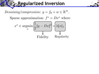
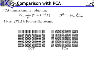
This document discusses sparse representations and dictionary learning. It introduces the concepts of sparsity, redundant dictionaries, and sparse coding. The goal of sparse coding is to find the sparsest representation of signals using an overcomplete dictionary. Dictionary learning aims to learn an optimized dictionary from exemplar data by alternately solving sparse coding subproblems and dictionary update steps. Patch-based dictionary learning has applications in image denoising and texture synthesis. In contrast to PCA, learned dictionaries contain non-linear atoms adapted to the data.