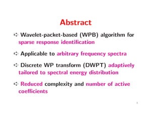
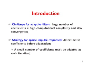
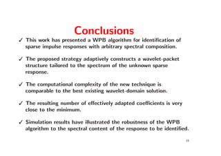
The document presents a wavelet-packet-based (wpb) algorithm aimed at identifying sparse impulse responses with arbitrary spectral energy distribution, focusing on reducing computational complexity and the number of adapted coefficients. The methodology includes an adaptive filtering strategy divided into two phases, and simulations demonstrate the algorithm's robustness compared to existing methods. Ultimately, the wpb algorithm effectively minimizes the number of adapted coefficients while maintaining competitive computational efficiency.

1. Abstract
Á Wavelet-packet-based (WPB) algorithm for
sparse response identification
Á Applicable to arbitrary frequency spectra
Á Discrete WP transform (DWPT) adaptively
tailored to spectral energy distribution
Á Reduced complexity and number of active
coefficients
1

2. Introduction
Challenge for adaptive filters: large number of
coefficients µ high computational complexity and slow
convergence;
Strategy for sparse impulse responses: detect active
coefficients before adaptation;
µ A small number of coefficients must be adapted at
each iteration;
2

3. Objectives in deriving the technique:
1. To enable the identification of sparse responses with
arbitrary spectral energy distribution;
2. To obtain a number of adaptive coefficients very
close to the number of nonzero samples of the
actual response;
3. To keep the computational complexity at levels
compatible with the competing algorithms.
3

4. Adaptation Strategy
Phase 1: Construction of the DWPT
PDWPT
z a2 (n) ˜
S z a (n)
HL 2 E
HH 2 z L3 (n) L
HH 2 E z (n)
˜
x(n) HH 2 C L3
z H3 (n) T
HL 2 I
˜
z a1 (n) O z H3 (n)
HL 2 N
˜
N ×N ˜
z a (n) y(n)
˜
wa (n)
-
˜
z L3 (n) y (n)
˜ e(n)
˜
wL3 (n)
+
˜
z H3 (n)
˜
wH3 (n)
4

5. Adaptation Strategy
Phase 1: Construction of the DWPT
y (n) → estimate of the desired signal y(n);
˜
e(n) → error y(n) − y (n);
˜
x(n) → N × 1 input vector for M-level DWPT (N = 2M );
H L and H H → low pass and high pass filters;
˜
z k (n) and z k (n) → transformed vectors
(k = a, a1, a2, L3, H3);
˜ ˜ ˜
wa(n), wL3 (n) and wH3 (n) → active weight vectors.
5

6. Adaptation Strategy
Phase 1: Construction of the DWPT
1st step: wH1 and wL1 adapted for few iterations;
2nd step: wH1 and wL1 compared against threshold
µ wH1 and wL1 ;
˜ ˜
3rd step: Next DWPT level subdivides subband of
the more energy.
Repeated for the number of DWPT levels.
6

7. Adaptation Strategy
Phase 2: Adaptation
m-th level adaptive weights below threshold are
deactivated. (m − 1)-th level adaptive weights in the
same temporal hierarchy of m-th level active weights
are activated (a little different for m = 1).
level m = 1
level m = 2
* level m = 3
level m = 4
}level m = 5
For each m, one adaptive filtering cycle.
7

8. Adaptation Strategy
Adaptive Filtering Structure: Phase 1
˜
z a(n) y(n)
P ˜
wa(n)
D z (n) -
x(n) ˜ Lm y (n)
˜ e(n)
W ˜
wLm (n)
P +
˜
T z Hm (n) ˜
wHm (n)
˜
N ×N
8

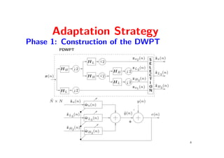
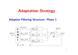
9. Adaptive Filtering Structure: Phase 1
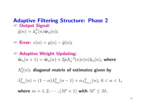
Output Signal:
y (n) = z T (n)w(n), where
˜ ˜ ˜
z (n) = [˜ T (n), z T m (n), z T m (n)]T ,
˜ za ˜L ˜H
w(n) = [wT (n), wT m (n), wT m (n)]T ;
˜ ˜a ˜L ˜H
Error: e(n) = y(n) − y (n);
˜
Adaptive Weight Updating:
˜ ˜
wa(n + 1) = wa(n) + 2˜Λ−2(n)e(n)˜ a(n)
µ a z
wLm (n + 1) = wLm (n) + 2˜λ−2 (n)e(n)˜ Lm (n)
˜ ˜ µ Lm z
wHm (n + 1) = wHm (n) + 2˜λ−2 (n)e(n)˜ Hm (n);
˜ ˜ µ Hm z
9

10. Adaptation Strategy
Adaptive Filtering Structure: Phase 2
d(n)
-
x(n) ˜
z a(n) y (n)
˜ e(n)
DWPT ˜
wa(n)
+
˜
N ×N
10

11. Adaptive Filtering Structure: Phase 2
Output Signal:
y (n) = z T (n)wa(n);
˜ ˜a ˜
Error: e(n) = y(n) − y (n);
˜
Adaptive Weight Updating:
˜ ˜
wa(n + 1) = wa(n) + 2˜Λ−2(n)e(n)˜ a(n), where
µ a z
Λ2 (n): diagonal matrix of estimates given by
a
λ2 m (n) = (1 − α)λ2 m (n − 1) + αzam,1 (n), 0 α 1,
a a
2
where m = 1, 2, · · · , (M ′ + 1) with M ′ ≤ M .
11

12. Computational Complexity
Definition:
˜
N : Number of coefficientes effectively adapted (NCEA).
Phase 1: Number of levels varies from 1 to M − 1
For a pass with (ℓ − 1) levels:
˜
(4N + 8ℓ − 3) operations and ℓ divisions.
Phase 2:
M levels:
˜
(4N + 8M + 5) operations and (M + 1) divisions.
12

13. Simulations
• Unknown responses: Sparse channel models from [6].
• Input signal: Generated using [5, Eq.(29)].
• Noise power: -40 dB
• Algorithms:
WPB - Wavelet-Packet-Based
HB - Haar-Basis [5]
TD-NLMS - Wavelet transformed NLMS
NLMS - Time-domain NLMS
13

14. • Detection thresholds:
˜˜
µξ(k)
T H = βf a
˜
λ2(k)
δ
˜ ˜ ˜
ξ(k) = (1 − µ)ξ(k − 1) + µe2(k)
˜ (Estimate of E[e2(k)])
βf a(phase 1 of WPB) = 3, 86
βf a(phase 2 of WPB) = 0, 77
βf a(HB) = 2.57, Pf a = 0.01
14

15. • Initial Adaptation Intervals for WPB
– Phase 1 - 1st band splitting: 6000 iterations
– Phase 1 - after activation/deactivation: 2000
iterations
1
– Phase 1 - all remaining AI’s: 16˜ iterations
µ
• Remaining Adaptation Intervals (AI)
1
– HB and WPB (Phase 2): 4˜
µ iterations
15

16. • Step sizes
1
– µN LM S = 8
1
– µT D−LM S = 8N (N = 512 - No. adaptive weights)
– µHB = 81ˆ
ˆ ˆ
(N - NCEA in HB)
N
– 1
µW P B = 10N
˜ ˜
(N - NCEA in WPB)
˜
16

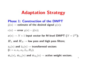
17. Simulation Results
Channel Response Model 1 [6]:
Number of Coefficients Normalized Mean-Square
Effectively Adapted Deviation
600 1
HB WPB
WPB −3 HB
500 TD-LMS
−7
NLMS
400 −11
MSD in dB
NCEA
−15
300
−19
200 −23
−27
100
−31
0 −35
0 40 80 120 160 200 240 280 320 0 40 80 120 160 200 240 280 320
3 3
iterations (×10 ) iterations (×10 )
17

18. Simulation Results
Channel Response Model 7 [6]:
Number of Coefficients Normalized Mean-Square
Effectively Adapted Deviation
600 10
HB WPB
WPB HB
500 TD-LMS
0
NLMS
400
MSD in dB
−10
NCEA
300
−20
200
−30
100
0 −40
0 40 80 120 160 200 240 280 320 0 40 80 120 160 200 240 280 320
3 3
iterations (×10 ) iterations (×10 )
18

19. Conclusions
This work has presented a WPB algorithm for identification of
sparse impulse responses with arbitrary spectral composition.
The proposed strategy adaptively constructs a wavelet-packet
structure tailored to the spectrum of the unknown sparse
response.
The computational complexity of the new technique is
comparable to the best existing wavelet-domain solution.
The resulting number of effectively adapted coefficients is very
close to the minimum.
Simulation results have illustrated the robustness of the WPB
algorithm to the spectral content of the response to be identified.
19

20. Bibliography
[1] Nurgun Erdol and Filiz Basbug, ”Wavelet Transform Based Adaptive Filters: Analysis and New
Results”, IEEE Transactions on Signal Processing, vol. 44, no. 9, pp. 2163 - 2171, Sept
1996.
[2] M. R. Petraglia and J. C. B. Torres, ”Performance Analysis of Adaptive Filter Structure
Employing Wavelet and Sparse Subfilters”, IEE Proceedings-Vision, Image and Signal
Processing, vol. 149, no. 2, pp. 115 - 119, April 2002.
[3] M. I. Doroslovacki and Howard Fan, ”Wavelet-Based Linear System Modeling and Adaptive
Filtering”, IEEE Trans. on Signal Proc., vol. 44, no. 5, pp. 1156 - 1167, May 1996.
[4] N. J. Bershad and A. Bist, ”Fast Coupled Adaptation for Sparse Impulse Responses Using a
Partial Haar Transform”, IEEE Trans. on Signal Proc., vol. 53, no. 3, pp. 966 - 976,
March 2005.
[5] K. C. Ho and S. D. Blunt, ”Rapid Identification of a Sparse Impulse Response Using an
Adaptive Algorithm in the Haar Domain”, IEEE Trans. on Signal Proc., vol. 51, no. 3, pp.
628-638, March 2003.
[6] Digital Network Echo Cancellers, ITU-T Recommendation G. 168, 2004.
[7] R. R. Coifman and Y. Meyer and M. V. Wickerhauser, Wavelet analysis and signal
processing, Jones and Barlett, Boston, 1992.
[8] St´phane Mallat, A wavelet tour of signal processing, Academic Press, 1998.
e
20