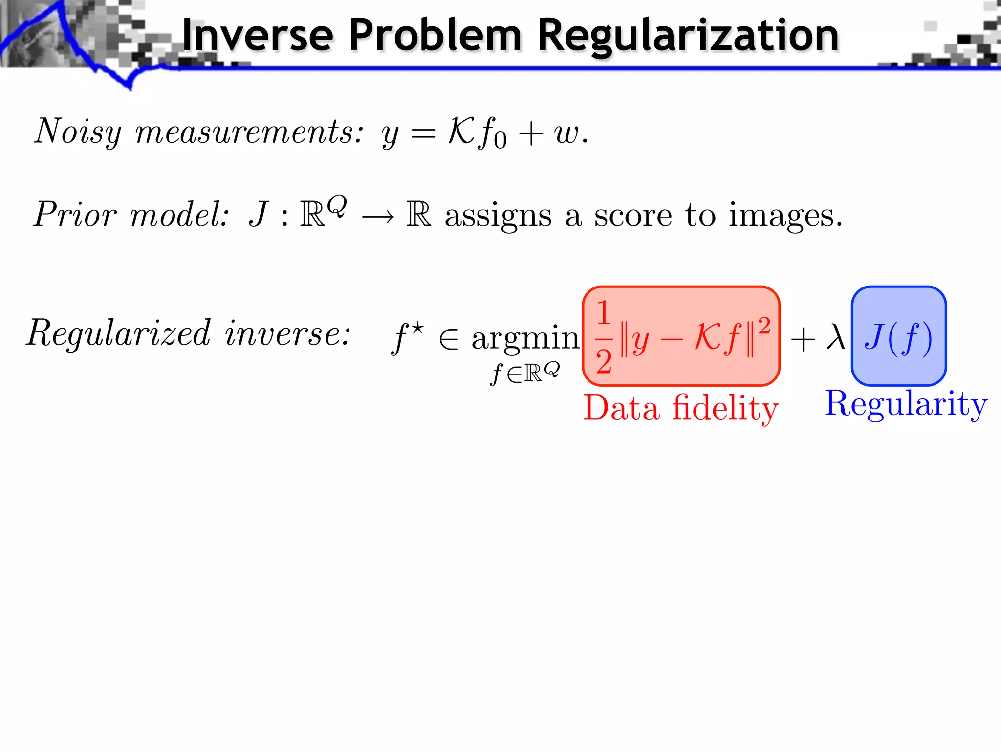
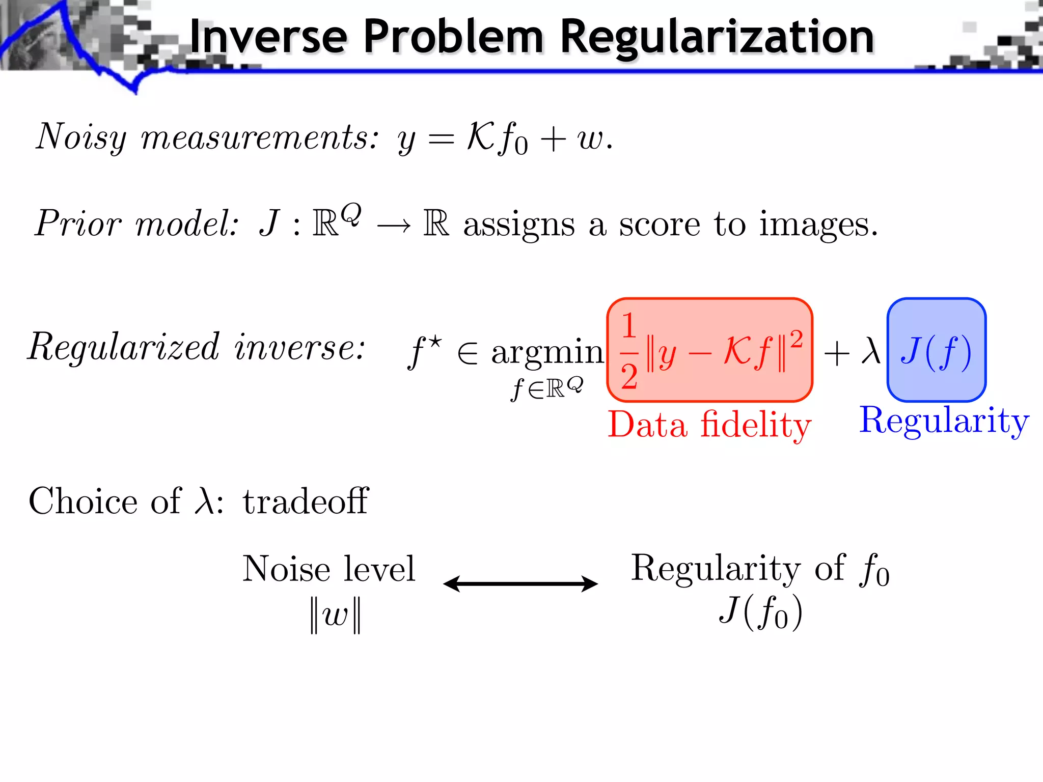
Downloaded 66 times


![Block Regularization
1 2
block sparsity: G(x) = ||x[b] ||, ||x[b] ||2 = x2
m
b B m b
iments Towards More Complex Penalization
(2) Bk
2
+ ` 1 `2
4
k=1 x 1,2
b B1 i b xi
⇥ x⇥⇥1 = i ⇥xi ⇥ b B i b xi2 +
i b xi
N: 256
b B2
b B
Image f = x Coe cients x.](https://image.slidesharecdn.com/2012-08-27-ismp-121213045802-phpapp02/75/A-Review-of-Proximal-Methods-with-a-New-One-40-2048.jpg)
![Block Regularization
1 2
block sparsity: G(x) = ||x[b] ||, ||x[b] ||2 = x2
m
b B m b
iments Towards More Complex Penalization
Non-overlapping decomposition: B = B ... B
Towards More Complex Penalization
Towards More Complex Penalization
n
1 n
2 G(x) =4 x iBk
(2)
+ ` ` k=1 G 1,2
(x) Gi (x) = ||x[b] ||,
1 2 i=1 b Bi
b b 1b1 B1 i b xiixb xi
22
BB
⇥ x⇥x⇥x⇥⇥1 =i ⇥x⇥x⇥xi ⇥
⇥= ++ +
i b i
⇥ ⇥1 ⇥1 = i i ⇥i i ⇥ bb B B i
Bb xii2bi2xi2
bbx
i
N: 256
b b 2b2 B2 i
BB xi2 b2xi
b b xi
i
b B
Image f = x Coe cients x. Blocks B1 B1 B2](https://image.slidesharecdn.com/2012-08-27-ismp-121213045802-phpapp02/75/A-Review-of-Proximal-Methods-with-a-New-One-41-2048.jpg)
![Block Regularization
1 2
block sparsity: G(x) = ||x[b] ||, ||x[b] ||2 = x2
m
b B m b
iments Towards More Complex Penalization
Non-overlapping decomposition: B = B ... B
Towards More Complex Penalization
Towards More Complex Penalization
n
1 n
2 G(x) =4 x iBk
(2)
+ ` ` k=1 G 1,2
(x) Gi (x) = ||x[b] ||,
1 2 i=1 b Bi
Each Gi is simple: b b 1b1 B1 i b xiixb xi
BB
22
⇥ x⇥x⇥x⇥⇥1 =i ⇥xG ⇥xi ⇥ m = b B B i b xii2bi2xi2
⇥ ⇥1 = i ⇥i i x +
i b i
⇤ m ⇥ b ⇥ Bi , ⇥ ⇥1Prox i ⇥xi ⇥(x) b max i0, 1
= Bb bx ++m
N: 256 ||x[b]b||B xi2 b2xi
2 2 B2
b B b i b b xi
i
b B
Image f = x Coe cients x. Blocks B1 B1 B2](https://image.slidesharecdn.com/2012-08-27-ismp-121213045802-phpapp02/75/A-Review-of-Proximal-Methods-with-a-New-One-42-2048.jpg)
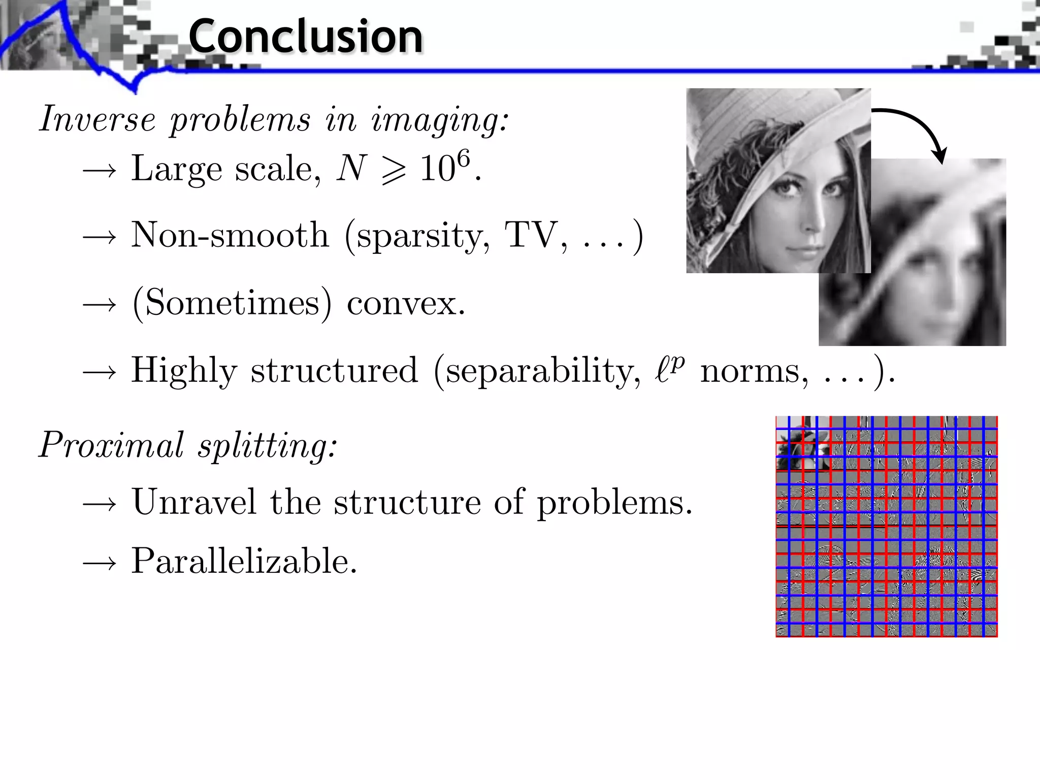

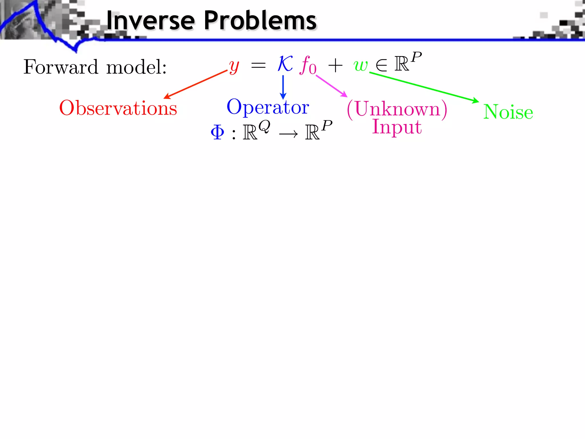
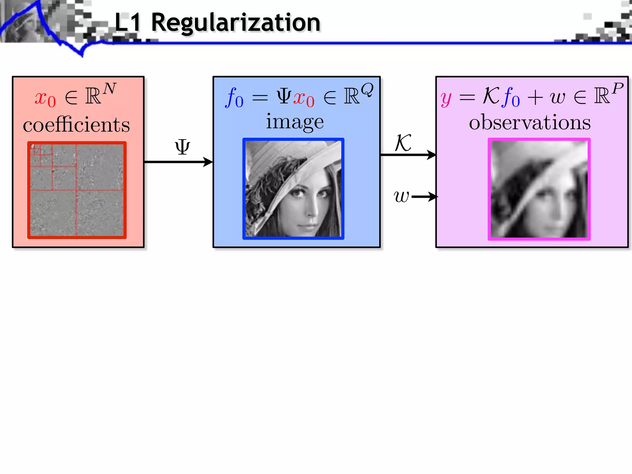
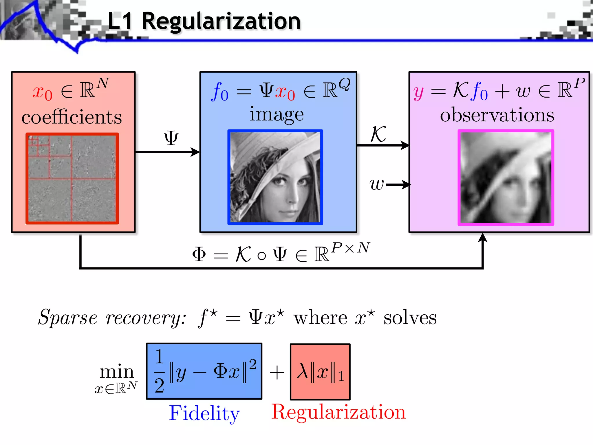
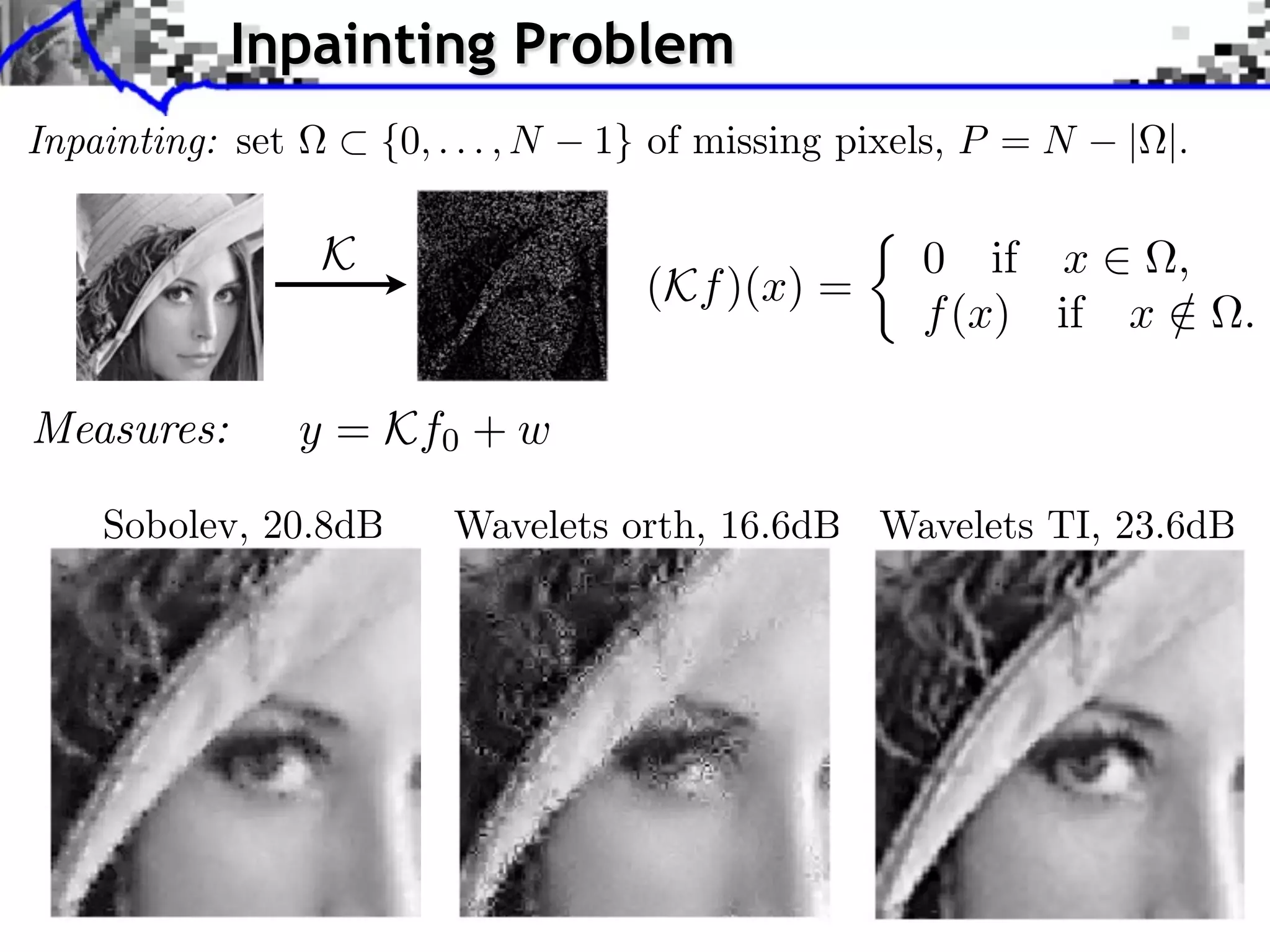
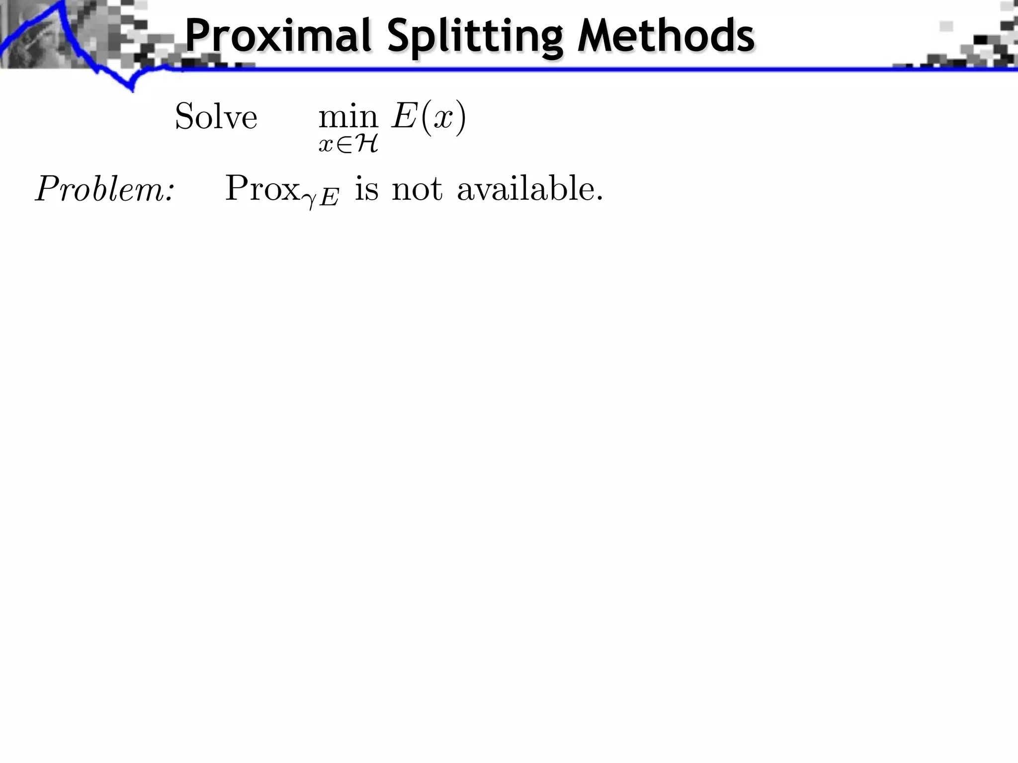
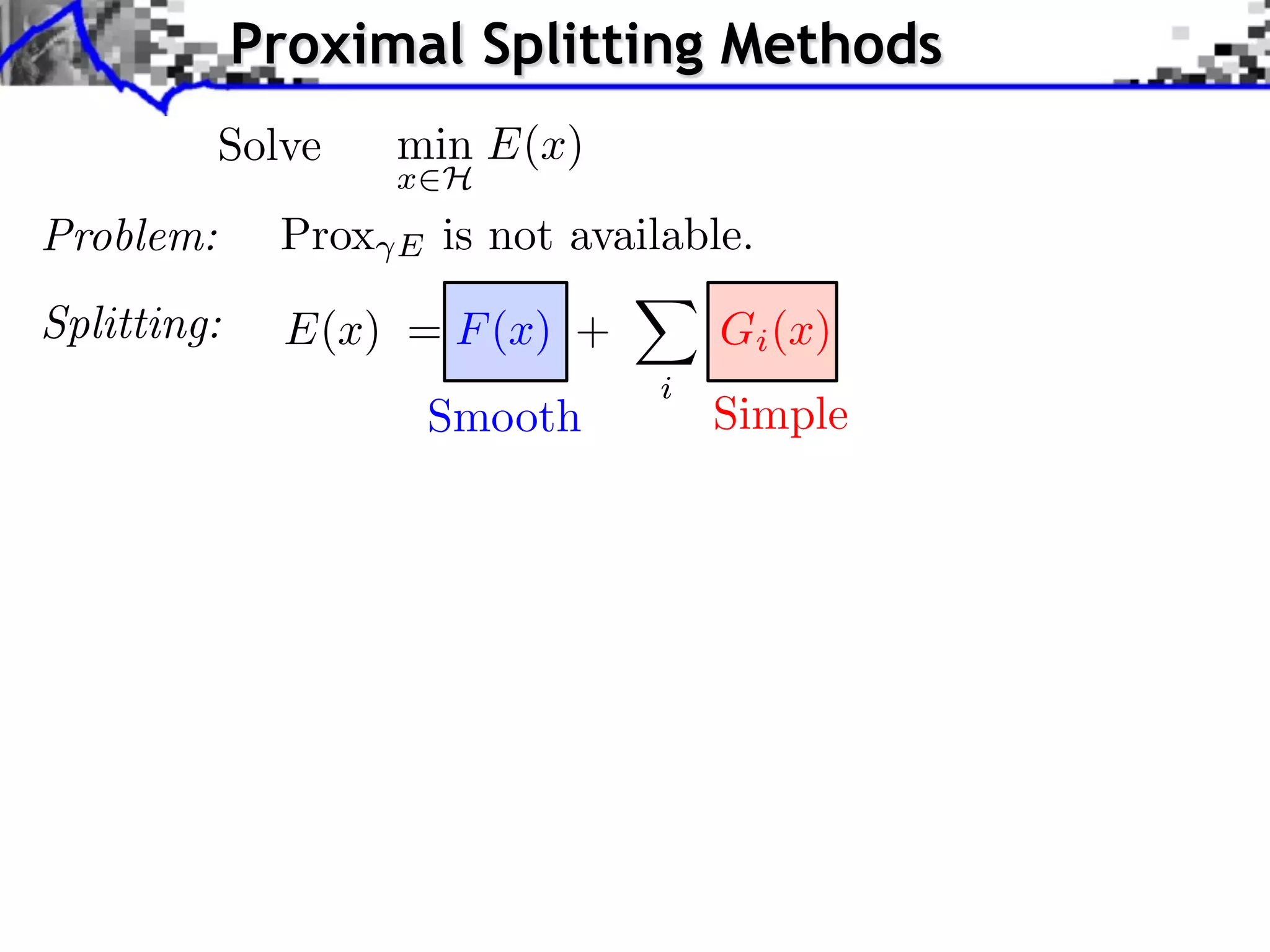
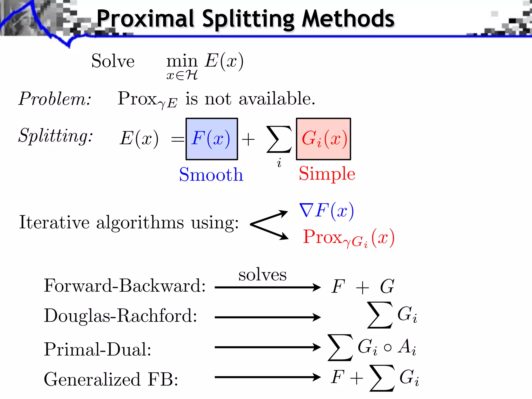
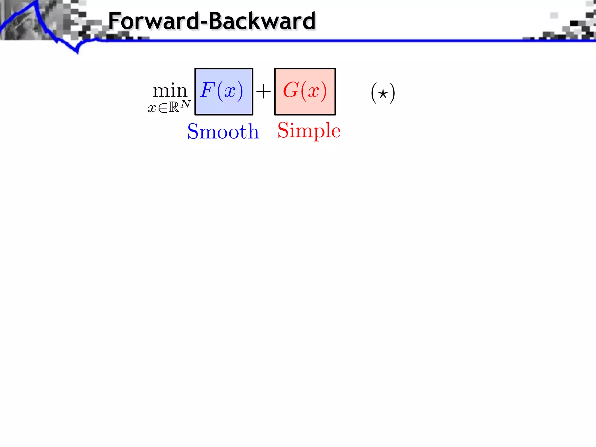
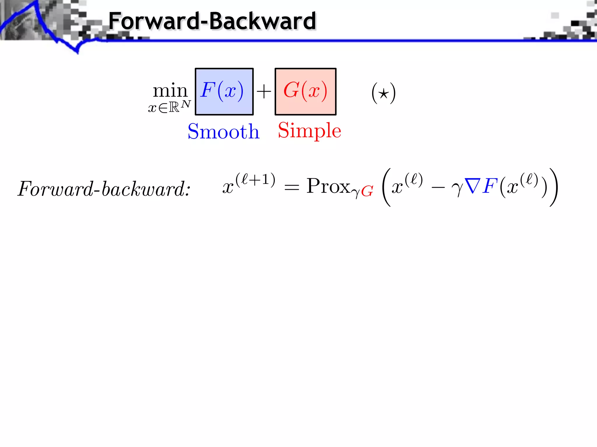
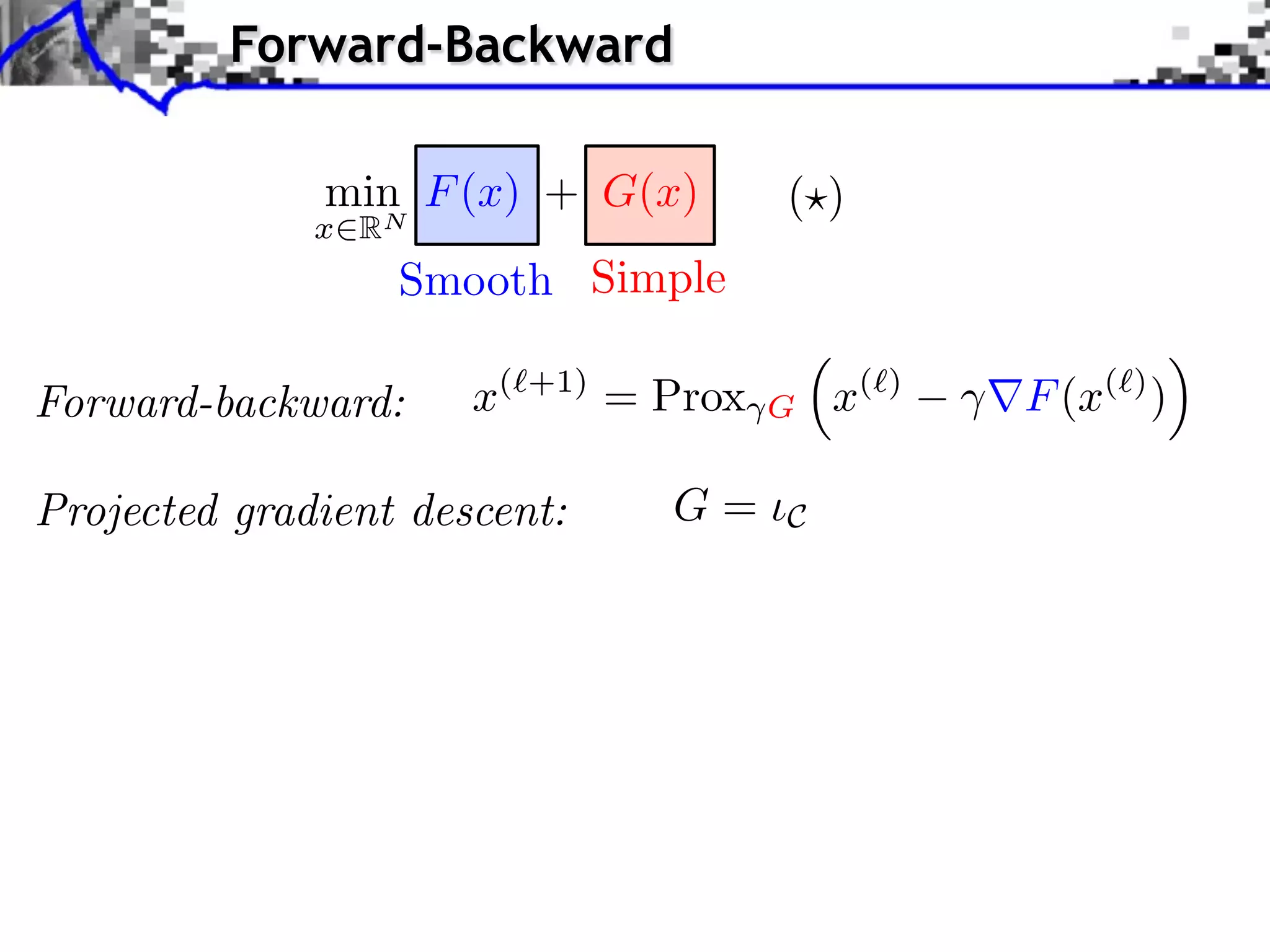
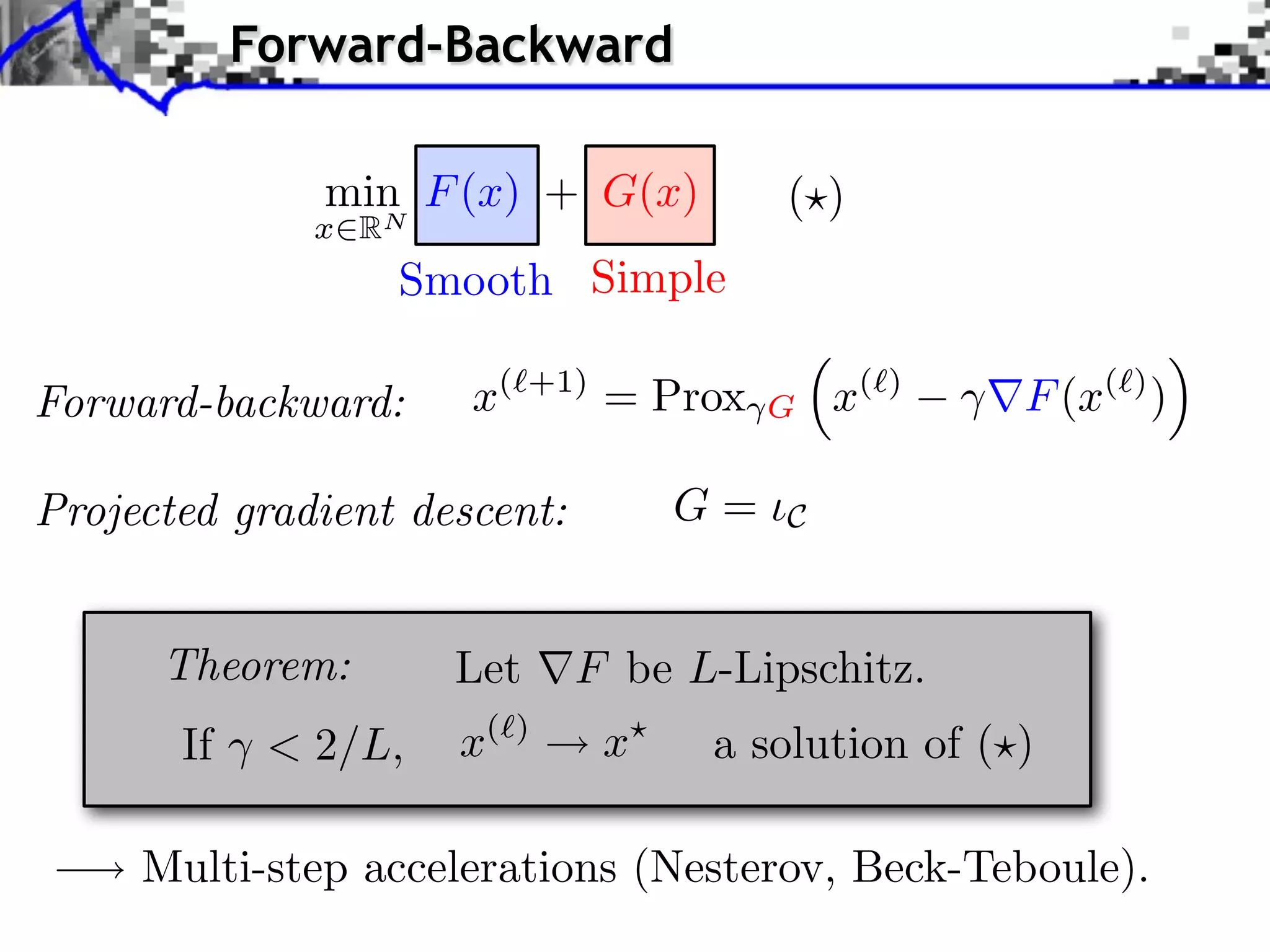
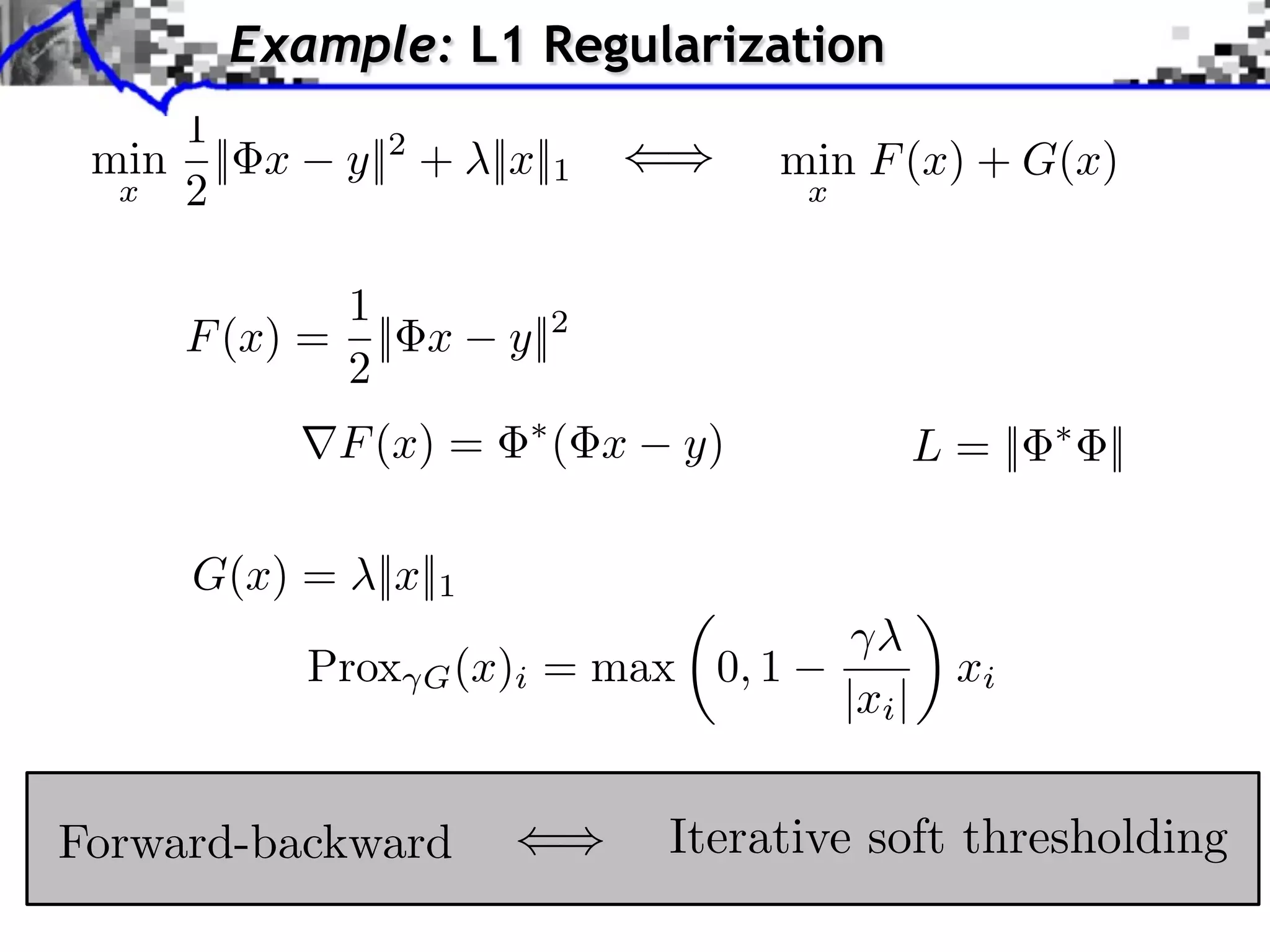
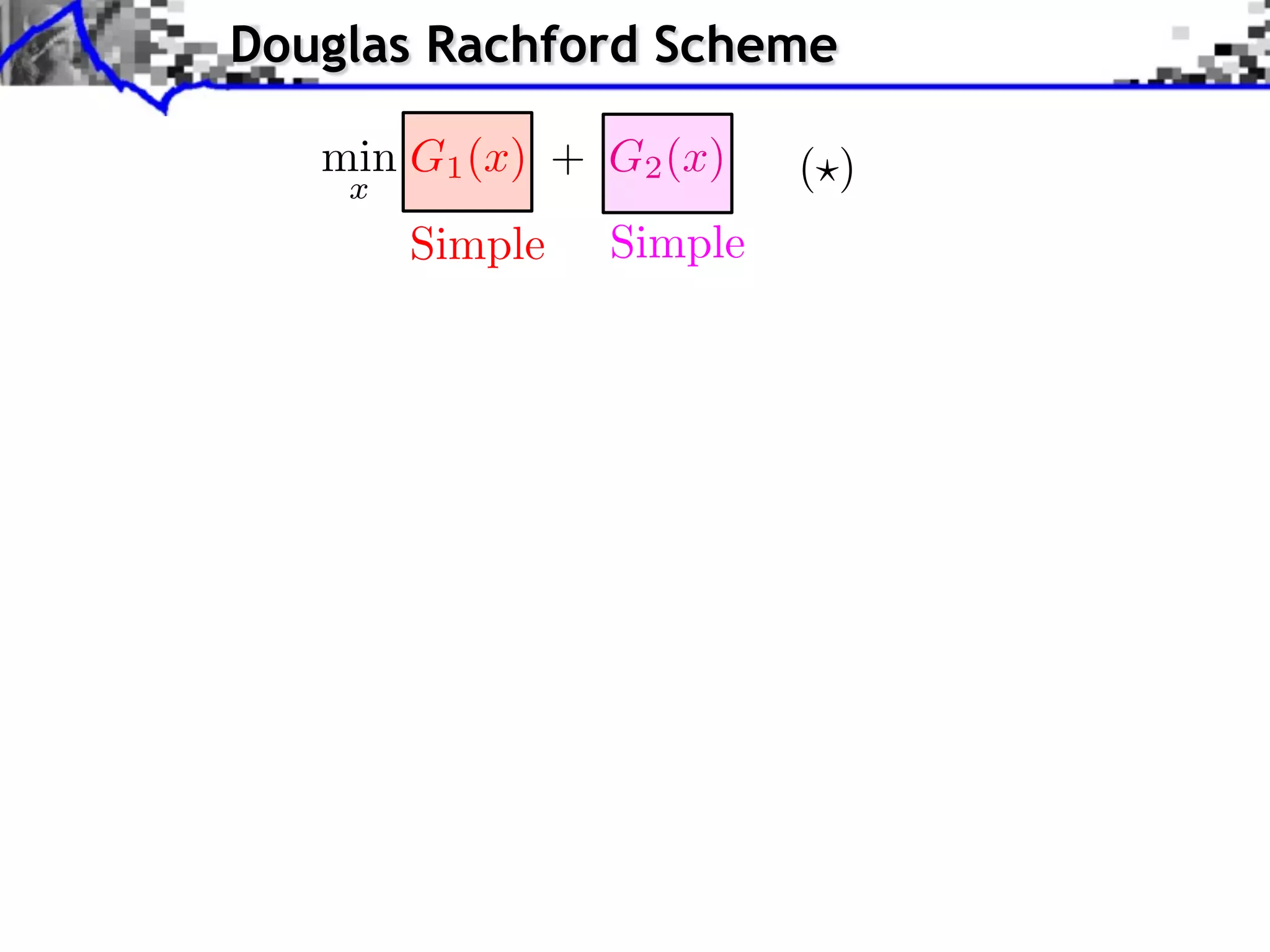
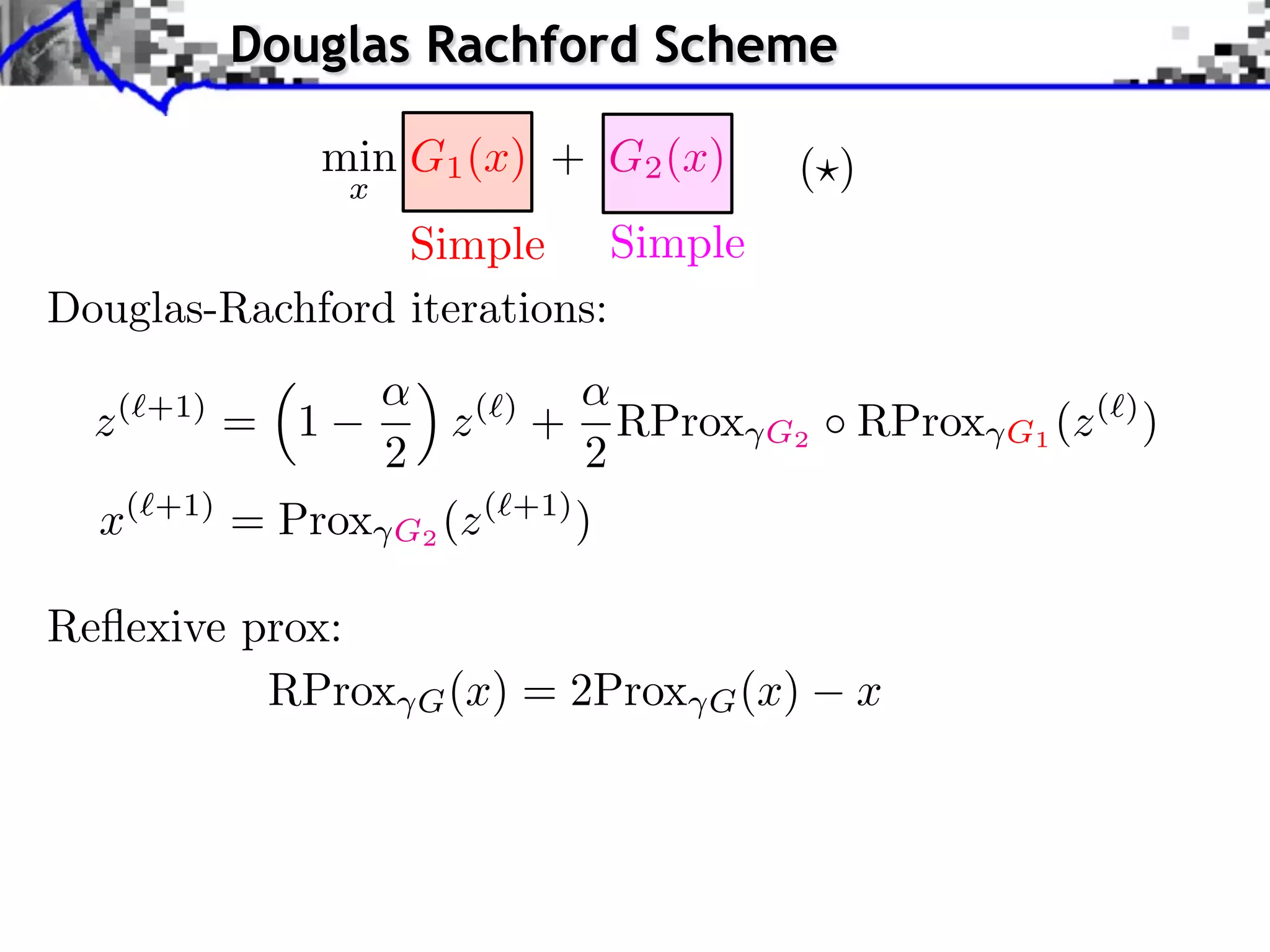
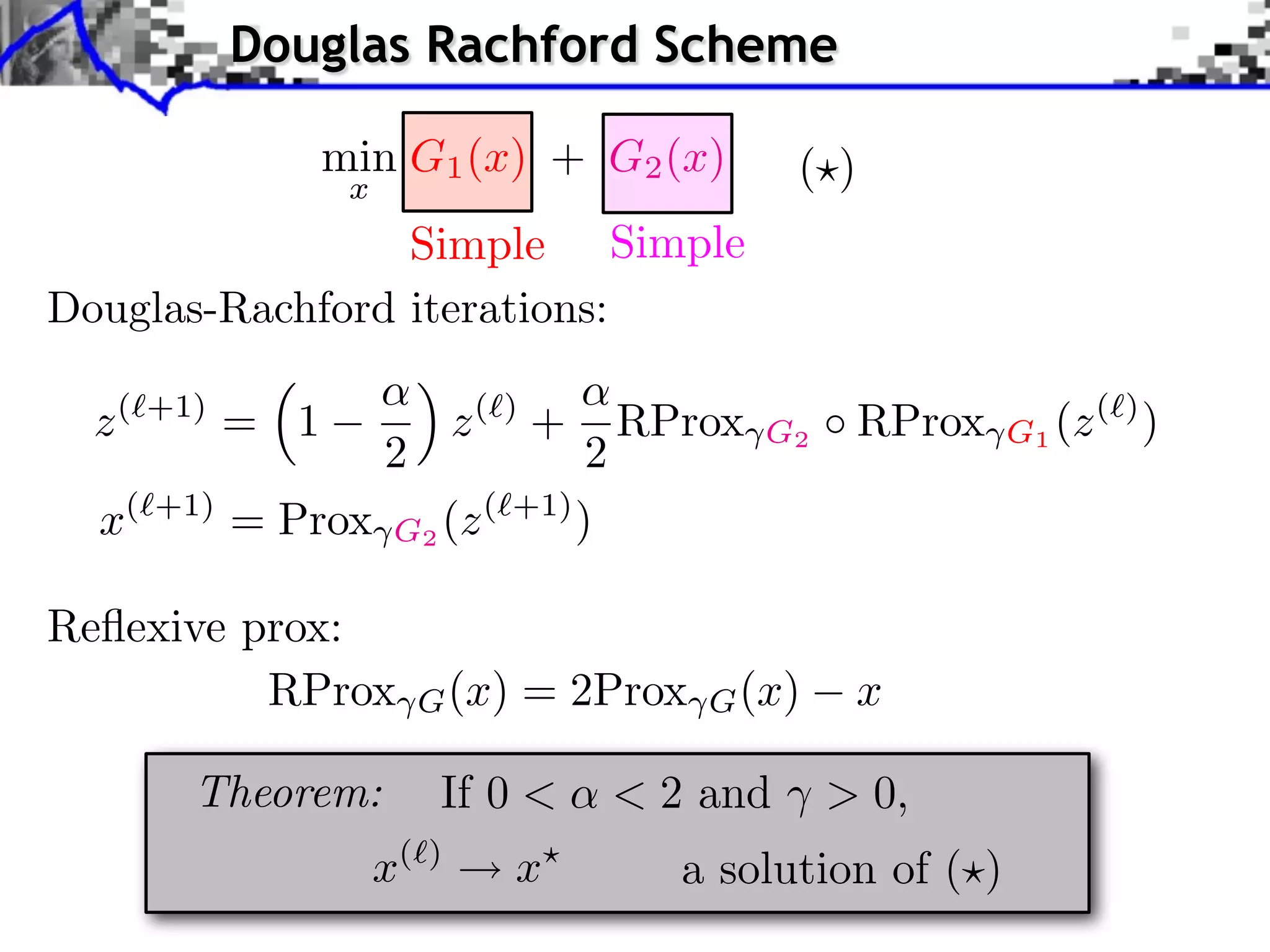
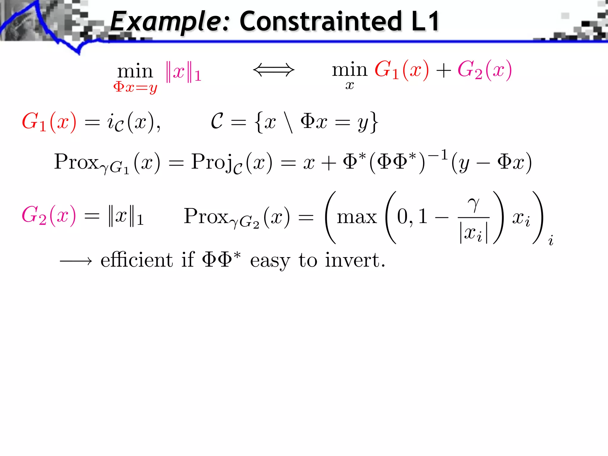
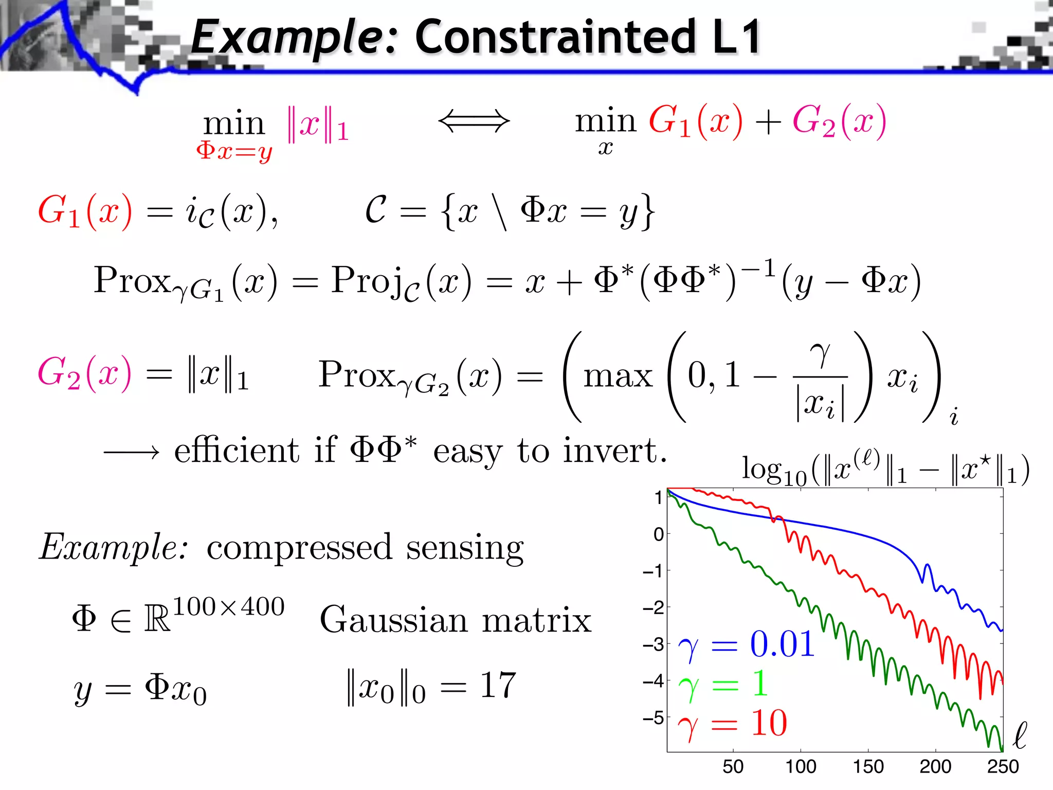
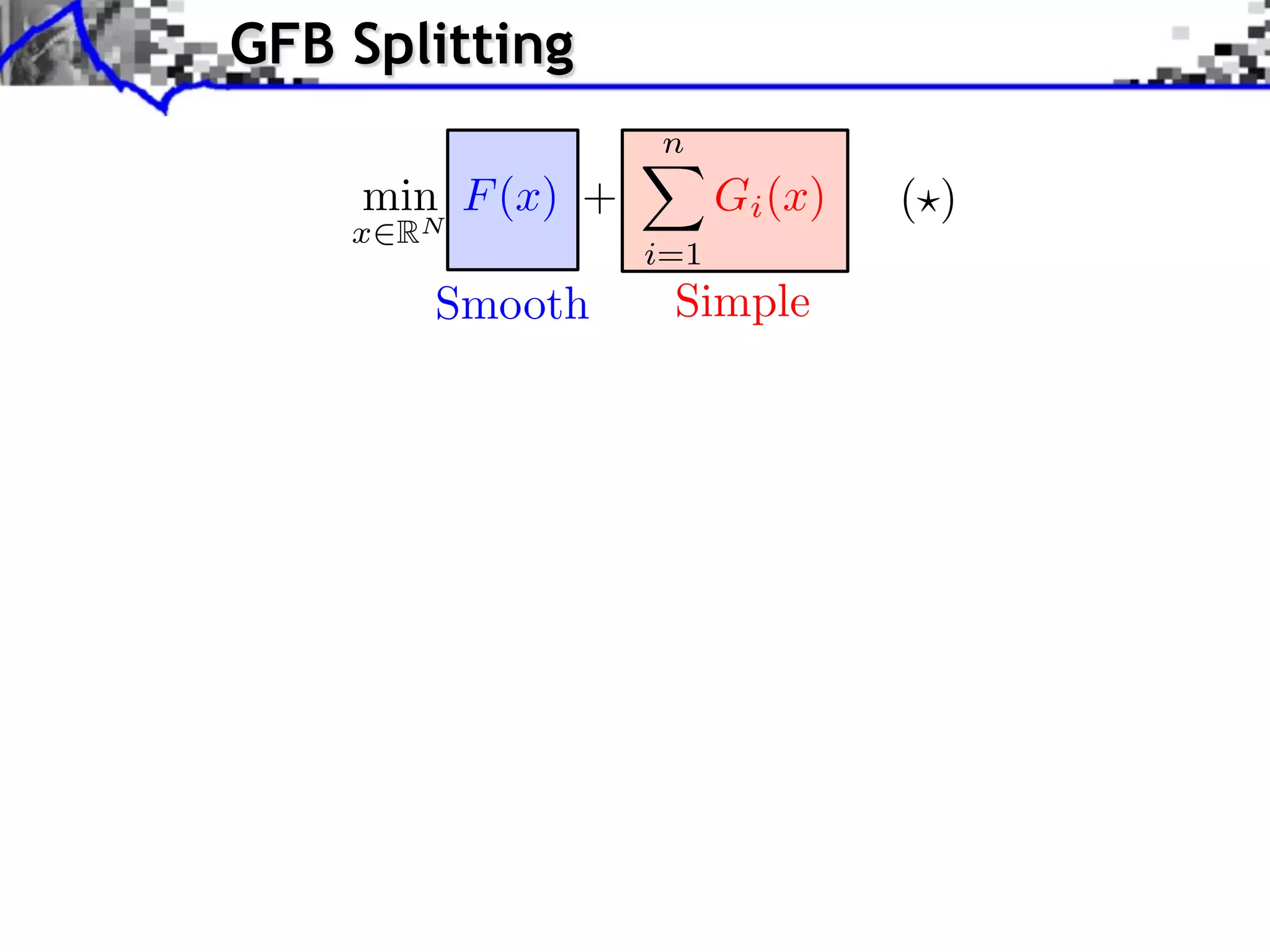
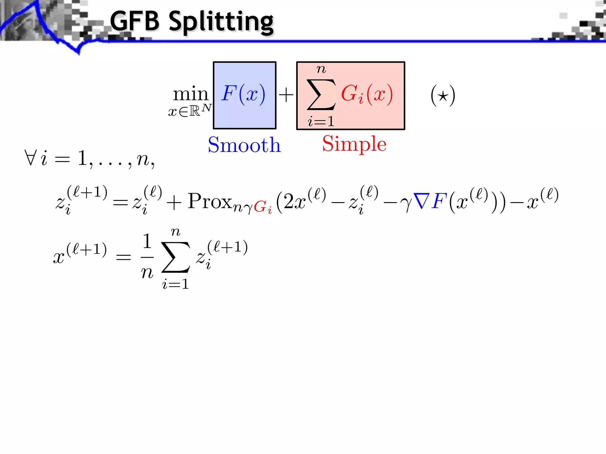
The document discusses proximal splitting methods for solving optimization problems with composite objectives. It begins by introducing inverse problems regularization and how proximal operators are used to solve problems by splitting them into smooth and non-smooth components. It then presents the forward-backward splitting method, Douglas-Rachford splitting, and the generalized forward-backward splitting method. Examples are provided to illustrate how these methods can be applied to problems like L1 regularization, constrained L1 minimization, and block sparsity regularization.