The document summarizes Rahul Singh's seminar presentation on reliability. It defines reliability as the ability of a product to perform as expected over time, with a probability between 0 and 1 under specified conditions. There are two types of failures: functional and reliability. Reliability is measured through failure rate and other metrics. Products go through debugging, chance failure, and wear-out phases as shown in the bathtub curve. Exponential and Weibull distributions model failure rates. System reliability depends on components arranged in series, parallel or both. Life testing plans include failure-terminated, time-terminated and sequential tests.

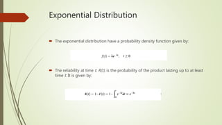
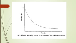
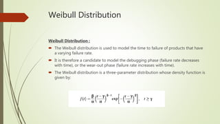
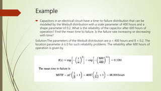
1. SEMINAR PRESENTATION
ON RELIABILITY
RAHUL SINGH
214218022

2. RELIABILITY
 Generally defined as the ability of a product to perform as expected over time.
 Formally defined as the probability that a product, piece of equipment, or system
performs its intended function for a stated period of time under specified
operating conditions.
 Although no product is expected to last forever, the time requirement ensures
satisfactory performance over at least a minimal stated period.

3. RELIABILITY
Four aspects of reliability are apparent from this definition:
• Reliability is a probability-related concept; the numerical value of this
probability is between 0 and 1.
• The functional performance of the product has to meet certain stipulations.
• Reliability implies successful operation over a certain period of
time.
• Operating or environmental conditions under which product use takes place are
specified.

4.  Types of Failures
 Functional failure – failure that occurs at the start of product life due to
manufacturing or material detects.
 Reliability failure – failure after some period of use.

5. RELIABILITY
 Types of Reliability
1) Inherent reliability – predicted by product design.
2) Achieved reliability – observed during use.
 Reliability Measurement
1) Failure rate – number of failures per unit time.
2) Alternative measures
a) Mean time to failure
b) Mean time between failures

6. LIFE-CYCLE CURVE
 Most products go through three distinct phases from product inception to wear-
out.
1. The debugging phase,
2. The chance-failure phase, and
3. The wear-out phase
 Figure 1 shows a typical life-cycle curve for which the failure rate is plotted as a
function of time. This curve is often referred to as the bathtub curve.

8. LIFE-CYCLE CURVE
 The debugging phase, also known as the infant-mortality phase, exhibits a drop in
the failure rate as initial problems identified during prototype testing are ironed
out.
 The chance failure phase, between times t1 and t2, is then encountered; failures
occur randomly and independently. This phase, in which the failure rate is constant,
typically represents the useful life of the product.
 Following this is the wear-out phase, in which an increase in the failure rate is
observed. Here, at the end of their useful life, parts age and wear out.

9. Probability Distributions to Model Failure
Rate
Exponential Distribution :
 The life-cycle curve shows the variation of the failure rate as a function of time.
 For the chance-failure phase, which represents the useful life of the product, the
failure rate is constant.
 As a result, the exponential distribution can be used to describe the time to failure
of the product for this phase.

10. Exponential Distribution
 The exponential distribution have a probability density function given by:
 The reliability at time t, R(t), is the probability of the product lasting up to at least
time t. It is given by:

12. Example
 An amplifier has an exponential time-to-failure distribution with a failure rate of 8%
per 1000 hours. What is the reliability of the amplifier at 5000hours? Find the mean
time to failure?
Solution:

13. Weibull Distribution
Weibull Distribution :
 The Weibull distribution is used to model the time to failure of products that have
a varying failure rate.
 It is therefore a candidate to model the debugging phase (failure rate decreases
with time), or the wear-out phase (failure rate increases with time).
 The Weibull distribution is a three-parameter distribution whose density function is
given by:

14. Weibull Distribution
 The reliability function for the Weibull distribution is given by
 The mean time to failure, as given by
 The failure-rate function r(t) for the Weibull time-to-failure probability distribution
is

15. Weibull Distribution
Figure shows the shape of the failure-rate function for the Weibull failure density function, for values of the parameter ß of 0.5, 1, and 3.5.

16. Example
 Capacitors in an electrical circuit have a time-to-failure distribution that can be
modeled by the Weibull distribution with a scale parameter of 400 hours and a
shape parameter of 0.2. What is the reliability of the capacitor after 600 hours of
operation? Find the mean time to failure. Is the failure rate increasing or decreasing
with time?
Solution:The parameters of the Weibull distribution are a = 400 hours and ß = 0.2. The
location parameter ã is 0 for such reliability problems. The reliability after 600 hours of
operation is given by

17. Example
 This function decreases with time. It would model components in the debugging
phase.

18. SYSTEM RELIABILITY
 Most products are made up of a number of components. The reliability of each
component and the configuration of the system consisting of these components
determines the system reliability (i.e., the reliability of the product).
 Systems with Components in Series
 Systems with Components in Parallel
 Systems with Components in Mix Configuration

19. Systems with Components in Series
 It is assumed that the components operate independent of each other.
 In general, if there are n components in series, where the reliability of the ith
component is denoted by Ri, the system reliability is
Rs = R1 x R2 x ... X Rn

20. Systems with Components in Series
 The system reliability decreases as the number of components in series increases.
 Although overdesign in each component improves reliability, its impact would be
offset by the number of components in series.
 Moreover, manufacturing capabilities and resource limitations restrict the
maximum reliability of any given component.
 Product redesign that reduces the number of components in series is a viable
alternative.

21. Systems with Components in Parallel
 System reliability can be improved by placing components in parallel. The
components are redundant; the system operates as long as at least one of the
components operates.
 The only time the system fails is when all the parallel components fail.
 All components are assumed to operate simultaneously.
 Examples of redundant components placed in parallel to improve the reliability of
the system abound. For instance, the braking mechanism is a critical system in the
automobile. Dual subsystems thus exist so that if one fails, the brakes still work

23. Systems with Components in Parallel
 Suppose that we have n components in parallel, with the reliability of the ith
component denoted by Ri=1, 2, ..., n. Assuming that the components operate
randomly and independently of each other, the probability of failure of each
component is given by
Fi = 1 - Ri
 Now, the system fails only if all the components fail. Thus, the probability of system
failure is

24. Systems with Components in Parallel
 The reliability of the system is the complement of Fs and is given by

25. Systems with Components in Series and in
Parallel
 Complex systems often consist of components that are both in series and in
parallel.
 Reliability calculations are based on the concepts discussed previously, assuming
that the components operate independently.

26. RELIABILITY AND LIFE TESTING PLANS
 Plans for reliability and life testing are usually destructive in nature. They involve
observing a sample of items until a certain number of failures occur, observing over
a certain period of time to record the number of failures, or a combination of both.
 Such testing is usually done at the prototype stage, which can be expensive
depending on the unit cost of the item.
 Testing is usually conducted under simulated conditions, but it should mimic the
actual operating conditions as closely as possible.

27. Types of Tests
1. Failure-Terminated Test
 In failure-terminated plans, the tests are terminated when a preassigned number of
failures occurs in the chosen sample. Lot acceptance is based on the accumulated
test time of the items when the test is terminated. One acceptance criterion
involves whether the estimated average life of the item exceeds a stipulated value.
2. Time-Terminated Test
 A time-terminated test is terminated when a preassigned time T is reached.
Acceptance of the lot is based on the observed number of failures r during the test
time. If the observed number of failures f exceeds a preassigned value r, the lot is
rejected; otherwise, the lot is accepted.

28. Types of Tests
3. Sequential Reliability :Test In sequential reliability testing, no prior decision is
made as to the number of failures or the time to conduct the test. Instead, the
accumulated results of the test are used to decide whether to accept the lot, reject
the lot, or continue testing.

29. THANK YOU!